Page 151 - Applied Numerical Methods Using MATLAB

140 INTERPOLATION AND CURVE FITTING
For simplicity, we consider a third-order polynomial
3 2
h(x) = H 3 x + H 2 x + H 1 x + H 0 (3.6.1)
matching just two points (x 0 ,y 0 ), (x 1 ,y 1 ) and having the specified first derivatives

y ,y at the points. We can obtain the four coefficients H 3 ,H 2 ,H 1 ,H 0 by solving

0 1
3 2
h(x 0 ) = H 3 x + H 2 x + H 1 x 0 + H 0 = y 0
0 0
3 2
h(x 1 ) = H 3 x + H 2 x + H 1 x 1 + H 0 = y 1
1 1
(3.6.2)
2

h (x 0 ) = 3H 3 x + 2H 2 x 0 + H 1 = y
0 0
2

h (x 1 ) = 3H 3 x + 2H 2 x 1 + H 1 = y
1 1
As an alternative, we approximate the specified derivatives at the data points by
their differences
h(x 0 + ε) − h(x 0 ) y 2 − y 0 h(x 1 ) − h(x 1 − ε) y 1 − y 3

y = = , y = =
0 1
ε ε ε ε
(3.6.3)
and find the Lagrange/Newton polynomial matching the four points

(x 0 ,y 0 ), (x 2 = x 0 + ε, y 2 = y 0 + y ε), (x 3 = x 1 − ε, y 3 = y 1 − y ε), (x 1 ,y 1 )
0 1
(3.6.4)
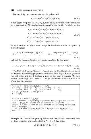
The MATLAB routine “hermit()” constructs Eq. (3.6.2) and solves it to get
the Hermite interpolating polynomial coefficients for a single interval given the
two end points and the derivatives at them as the input arguments. The next
routine “hermits()”uses “hermit()” to get the Hermite coefficients for a set
of multiple subintervals.
function H = hermit(x0,y0,dy0,x1,y1,dy1)
A = [x0^3 x0^2 x0 1; x1^3 x1^2 x1 1;
3*x0^2 2*x0 1 0; 3*x1^2 2*x1 1 0];
b = [y0 y1 dy0 dy1]’; %Eq.(3.6-2)
H=(A\b)’;
function H = hermits(x,y,dy)
% finds Hermite interpolating polynomials for multiple subintervals
%Input : [x,y],dy - points and derivatives at the points
%Output: H = coefficients of cubic Hermite interpolating polynomials
for n = 1:length(x)-1
H(n,:) = hermit(0,y(n),dy(n),x(n + 1)-x(n),y(n + 1),dy(n + 1));
end

Example 3.4. Hermite Interpolating Polynomial. Consider the problem of find-
ing the polynomial interpolation for the N + 1 = 4 data points

{(0, 0), (1, 1), (2, 4), (3, 5)} (E3.4.1)