Page 148 - Applied Numerical Methods Using MATLAB

INTERPOLATION BY CUBIC SPLINE 137

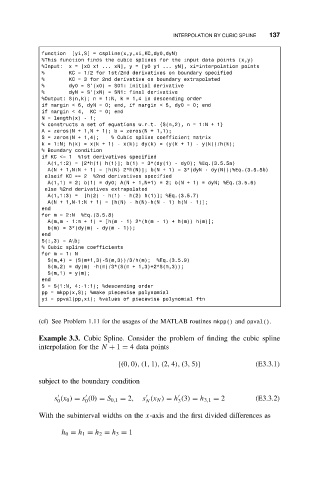
function [yi,S] = cspline(x,y,xi,KC,dy0,dyN)
%This function finds the cubic splines for the input data points (x,y)
%Input: x = [x0 x1 ... xN], y = [y0 y1 ... yN], xi=interpolation points
% KC = 1/2 for 1st/2nd derivatives on boundary specified
% KC = 3 for 2nd derivative on boundary extrapolated
% dy0 = S’(x0) = S01: initial derivative
% dyN = S’(xN) = SN1: final derivative
%Output: S(n,k); n = 1:N, k = 1,4 in descending order
if nargin < 6, dyN = 0; end, if nargin < 5, dy0 = 0; end
if nargin < 4, KC = 0; end
N = length(x) - 1;
% constructs a set of equations w.r.t. {S(n,2),n=1:N+1}
A = zeros(N + 1,N + 1); b = zeros(N + 1,1);
S = zeros(N + 1,4); % Cubic spline coefficient matrix
k = 1:N; h(k) = x(k + 1) - x(k); dy(k) = (y(k + 1) - y(k))/h(k);
% Boundary condition
if KC <= 1 %1st derivatives specified
A(1,1:2) = [2*h(1) h(1)]; b(1) = 3*(dy(1) - dy0); %Eq.(3.5.5a)
A(N + 1,N:N + 1) = [h(N) 2*h(N)]; b(N + 1) = 3*(dyN - dy(N));%Eq.(3.5.5b)
elseif KC == 2 %2nd derivatives specified
A(1,1) = 2; b(1) = dy0; A(N + 1,N+1) = 2; b(N + 1) = dyN; %Eq.(3.5.6)
else %2nd derivatives extrapolated
A(1,1:3) = [h(2) - h(1) - h(2) h(1)]; %Eq.(3.5.7)
A(N + 1,N-1:N + 1) = [h(N) - h(N)-h(N - 1) h(N - 1)];
end
for m = 2:N %Eq.(3.5.8)
A(m,m - 1:m + 1) = [h(m - 1) 2*(h(m - 1) + h(m)) h(m)];
b(m) = 3*(dy(m) - dy(m - 1));
end
S(:,3) = A\b;
% Cubic spline coefficients
form=1:N
S(m,4) = (S(m+1,3)-S(m,3))/3/h(m); %Eq.(3.5.9)
S(m,2) = dy(m) -h(m)/3*(S(m + 1,3)+2*S(m,3));
S(m,1) = y(m);
end
S = S(1:N, 4:-1:1); %descending order
pp = mkpp(x,S); %make piecewise polynomial
yi = ppval(pp,xi); %values of piecewise polynomial ftn

(cf) See Problem 1.11 for the usages of the MATLAB routines mkpp() and ppval().

Example 3.3. Cubic Spline. Consider the problem of finding the cubic spline
interpolation for the N + 1 = 4 data points

{(0, 0), (1, 1), (2, 4), (3, 5)} (E3.3.1)

subject to the boundary condition

s (x 0 ) = s (0) = S 0,1 = 2, s (x N ) = h (3) = h 3,1 = 2 (E3.3.2)
0 0 N 3
With the subinterval widths on the x-axis and the first divided differences as
h 0 = h 1 = h 2 = h 3 = 1