Page 145 - Applied Numerical Methods Using MATLAB

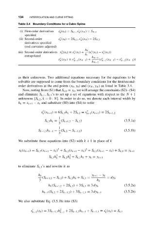
134 INTERPOLATION AND CURVE FITTING
Table 3.4 Boundary Conditions for a Cubic Spline

(i) First-order derivatives s (x 0 ) = S 0,1 ,s (x N ) = S N,1

0
N
specified
(ii) Second-order s (x 0 ) = 2S 0,2 ,s (x N ) = 2S N,2

N
0
derivatives specified
(end-curvature adjusted)
h 0

(iii) Second-order derivatives s (x 0 ) ≡ s (x 1 ) + (s (x 1 ) − s (x 2 ))
0 1 1 2
extrapolated h 1
h N−1

s (x N ) ≡ s N−1 (x N−1 ) + (s N−1 (x N−1 ) − s N−2 (x N−2 ))

N
h N−2
as their unknowns. Two additional equations necessary for the equations to be
solvable are supposed to come from the boundary conditions for the first/second-
order derivatives at the end points (x 0 ,y 0 )and (x N ,y N ) as listed in Table 3.4.
Now, noting from (S1) that S k,0 = y k , we will arrange the constraints (S2)–(S4)
and eliminate S k,1 ,S k,3 ’s to set up a set of equations with respect to the N + 1
unknowns {S k,2 ,k = 0: N}. In order to do so, we denote each interval width by
h k = x k+1 − x k and substitute (S0) into (S4) to write
s (x k+1 ) = 6S k,3 h k + 2S k,2 ≡ s

k k+1 (x k+1 ) = 2S k+1,2
1
S k,3 h k = (S k+1,2 − S k,2 ) (3.5.1a)
3
1
S k−1,3 h k−1 = (S k,2 − S k−1,2 ) (3.5.1b)
3
We substitute these equations into (S2) with k + 1inplace of k
3 2
s k (x k+1 ) = S k,3 (x k+1 − x k ) + S k,2 (x k+1 − x k ) + S k,1 (x k+1 − x k ) + S k,0 ≡ y k+1
3 2
S k,3 h + S k,2 h + S k,1 h k + y k ≡ y k+1
k k
to eliminate S k,3 ’s and rewrite it as

h k y k+1 − y k
(S k+1,2 − S k,2 ) + S k,2 h k + S k,1 = = dy k
3 h k
(3.5.2a)
h k (S k+1,2 + 2S k,2 ) + 3S k,1 = 3 dy k
(3.5.2b)
h k−1 (S k,2 + 2S k−1,2 ) + 3S k−1,1 = 3 dy k−1
We also substitute Eq. (3.5.1b) into (S3)

s (x k ) = 3S k−1,3 h 2 + 2S k−1,2 h k−1 + S k−1,1 ≡ s (x k ) = S k,1
k−1 k−1 k