Page 342 - Applied Numerical Methods Using MATLAB

UNCONSTRAINED OPTIMIZATION 331
This algorithm is essentially to find the zero of the gradient function g(x) of the
objective function and consequently, it can be implemented by using any vector
nonlinear equation solver. What we have to do is just to define the gradient
function g(x) and put the function name as an input argument of any routine
like “newtons()”or “fsolve()” for solving a system of nonlinear equations
(see Section 4.6).
Now, we make a MATLAB program “nm715.m”, which actually solves
g(x) = 0 for the gradient function

T

∂f ∂f
g(x) =∇f(x) = = 2x 1 − x 2 − 4 2x 2 − x 1 − 1 (7.1.14)
∂x 1 ∂x 2
of the objective function (7.1.6)
2 2
f(x) = f(x 1 ,x 2 ) = x − x 1 x 2 − 4x 1 + x − x 2
1 2
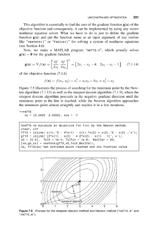
Figure 7.5 illustrates the process of searching for the minimum point by the New-
ton algorithm (7.1.13) as well as the steepest descent algorithm (7.1.9), where the
steepest descent algorithm proceeds in the negative gradient direction until the
minimum point in the line is reached, while the Newton algorithm approaches
the minimum point almost straightly and reaches it in a few iterations.

>>nm715
xo = [3.0000 2.0000], ans = -7

%nm715 to minimize an objective ftn f(x) by the Newton method.
clear, clf
f713 = inline(’x(1).^2 - 4*x(1) - x(1).*x(2) + x(2).^2 - x(2)’,’x’);
g713 = inline(’[2*x(1) - x(2) - 4 2*x(2) - x(1) - 1]’,’x’);
x0 = [0 0], TolX = 1e-4; TolFun = 1e-6; MaxIter = 50;
[xo,go,xx] = newtons(g713,x0,TolX,MaxIter);
xo, f713(xo) %an extremum point reached and its function value

4

3

2

1 Newton

steepest descent
0
0 1 2 3 4 5 6
Figure 7.5 Process for the steepest descent method and Newton method (‘‘nm714.m’’ and
‘‘nm715.m’’).