Page 347 - Applied Numerical Methods Using MATLAB

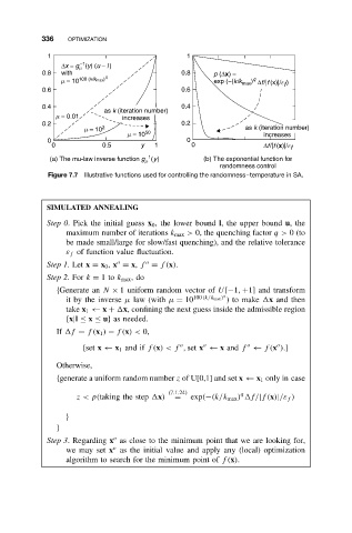
336 OPTIMIZATION
1 1
−1
∆x = g (y) (u − l )

m
0.8 with q 0.8 p (∆x) =
m = 10 100 (k/k max ) exp (−(k/k max ) q ∆f/|f (x)|/e )
f
0.6 0.6
0.4 0.4
as k (iteration number)
m = 0.01 increases
0.2 0.2
m = 10 2 as k (iteration number)
m = 10 50 increases
0 0
0 0.5 y 1 0 ∆f/|f (x)|/e f
−1
(a) The mu-law inverse function g (y) (b) The exponential function for
m
randomness control
Figure 7.7 Illustrative functions used for controlling the randomness–temperature in SA.
SIMULATED ANNEALING
Step 0. Pick the initial guess x 0 , the lower bound l, the upper bound u,the
maximum number of iterations k max > 0, the quenching factor q> 0(to
be made small/large for slow/fast quenching), and the relative tolerance
ε f of function value fluctuation.
o
o
Step 1.Let x = x 0 , x = x, f = f(x).
Step 2.For k = 1to k max ,do
{Generate an N × 1 uniform random vector of U[−1, +1] and transform
it by the inverse µ law (with µ = 10 100 (k/k max ) q )tomake x and then
take x 1 ← x + x, confining the next guess inside the admissible region
{x|l ≤ x ≤ u} as needed.
If f = f(x 1 ) − f(x)< 0,

o o o o
{set x ← x 1 and if f(x)<f , set x ← x and f ← f(x ).}
Otherwise,
{generate a uniform random number z of U[0,1] and set x ← x 1 only in case
(7.1.24) q
z<p(taking the step x) = exp(−(k/k max ) f/|f(x)|/ε f )

}
}
o
Step 3. Regarding x as close to the minimum point that we are looking for,
o
we may set x as the initial value and apply any (local) optimization
algorithm to search for the minimum point of f(x).