Page 345 - Applied Numerical Methods Using MATLAB

334 OPTIMIZATION
Based on the fact that minimizing this quadratic objective function is equivalent
to solving the linear equation
g(x) =∇f(x) = Hx + b = 0 (7.1.20)

MATLAB has several built-in routines such as “cgs()”,“pcg()”, and “bicg()”,
which use the conjugate gradient method to solve a set of linear equations.
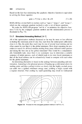
We make the MATLAB program “nm716.m” to minimize the objective func-
tion (7.1.6) by the conjugate gradient method and the minimization process is
illustrated in Fig. 7.6.

7.1.7 Simulated Annealing Method [W-7]
All of the optimization methods discussed so far may be more or less efficient
in finding the minimum point if only they start from the initial point sufficiently
close to it. But, the point they reach may be one of several local minima and we
often cannot be sure that it is the global minimum. How about repeating the pro-
cedure to search for all local minima starting from many different initial guesses
and taking the best one as the global minimum? This would be a computation-
ally formidable task, since there is no systematic way to determine a suitable
sequence of initial guesses, each of which leads to its own (local) minimum so
that all the local minima can be exhaustively found to compete with each other
for the global minimum.
An interesting alternative is based on the analogy between annealing and min-
imization. Annealing is the physical process of heating up a solid metal above its
melting point and then cooling it down so slowly that the highly excited atoms
can settle into a (global) minimum energy state, yielding a single crystal with
a regular structure. Fast cooling by rapid quenching may result in widespread

4

3

2

1

0
0 1 2 3 4 5 6
Figure 7.6 Process for the conjugate gradient method (‘‘nm716.m’’).