Page 47 - Applied Numerical Methods Using MATLAB

36 MATLAB USAGE AND COMPUTATIONAL ERRORS
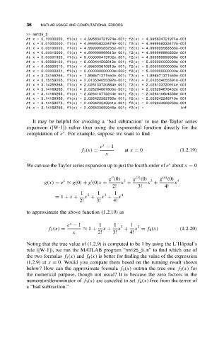
>> nm125_2
At x = 0.10000000, f1(x) = 4.995834721974e-001; f2(x) = 4.995834721974e-001
At x = 0.01000000, f1(x) = 4.999958333474e-001; f2(x) = 4.999958333472e-001
At x = 0.00100000, f1(x) = 4.999999583255e-001; f2(x) = 4.999999583333e-001
At x = 0.00010000, f1(x) = 4.999999969613e-001; f2(x) = 4.999999995833e-001
At x = 0.00001000, f1(x) = 5.000000413702e-001; f2(x) = 4.999999999958e-001
At x = 0.00000100, f1(x) = 5.000444502912e-001; f2(x) = 5.000000000000e-001
At x = 0.00000010, f1(x) = 4.996003610813e-001; f2(x) = 5.000000000000e-001
At x = 0.00000001, f1(x) = 0.000000000000e+000; f2(x) = 5.000000000000e-001
At x = 3.24159265, f1(x) = 1.898571371550e-001; f2(x) = 1.898571371550e-001
At x = 3.15159265, f1(x) = 2.013534055392e-001; f2(x) = 2.013534055391e-001
At x = 3.14259265, f1(x) = 2.025133720884e-001; f2(x) = 2.025133720914e-001
At x = 3.14169265, f1(x) = 2.026294667803e-001; f2(x) = 2.026294678432e-001
At x = 3.14160265, f1(x) = 2.026410772244e-001; f2(x) = 2.026410604538e-001
At x = 3.14159365, f1(x) = 2.026422382785e-001; f2(x) = 2.026242248740e-001
At x = 3.14159275, f1(x) = 2.026423543841e-001; f2(x) = 2.028044503269e-001
At x = 3.14159266, f1(x) = 2.026423659946e-001; f2(x) = Inf

It may be helpful for avoiding a ‘bad subtraction’ to use the Taylor series
expansion ([W-1]) rather than using the exponential function directly for the
x
computation of e . For example, suppose we want to find
x
e − 1
f 3 (x) = at x = 0 (1.2.19)
x
x
We can use the Taylor series expansion up to just the fourth-order of e about x = 0
(3)
(4)

g (0) g (0) g (0)
x 2 3 4
g(x) = e ≈ g(0) + g (0)x + x + x + x
2! 3! 4!
1 2 1 3 1 4
= 1 + x + x + x + x
2! 3! 4!
to approximate the above function (1.2.19) as
x
e − 1 1 1 2 1 3
f 3 (x) = ≈ 1 + x + x + x = f 4 (x) (1.2.20)
x 2! 3! 4!
Noting that the true value of (1.2.9) is computed to be 1 by using the L’Hˆ opital’s
rule ([W-1]), we run the MATLAB program “nm125_3.m” to find which one of
the two formulas f 3 (x) and f 4 (x) is better for finding the value of the expression
(1.2.9) at x = 0. Would you compare them based on the running result shown
below? How can the approximate formula f 4 (x) outrun the true one f 3 (x) for
the numerical purpose, though not usual? It is because the zero factors in the
numerator/denominator of f 3 (x) are canceled to set f 4 (x) free from the terror of
a “bad subtraction.”