Page 49 - Applied Numerical Methods Using MATLAB

38 MATLAB USAGE AND COMPUTATIONAL ERRORS
polynomial
4 3 2
p 4 (x) = a 1 x + a 2 x + a 3 x + a 4 x + a 5 (1.3.1)

It is better to use the nested structure (as below) than to use the above form as
it is.
p 4n (x) = (((a 1 x + a 2 )x + a 3 )x + a 4 )x + a 5 (1.3.2)
Note that the numbers of multiplications needed in Eqs. (1.3.2) and (1.3.1) are
4and (4 + 3 + 2 + 1 = 9), respectively. This point is illustrated by the program
N−1 i 6
“nm131_1.m”, where a polynomial a i x of degree N = 10 for a certain
i=0
value of x is computed by using the three methods—that is, Eq. (1.3.1), Eq.
(1.3.2), and the MATLAB built-in function ‘polyval()’. Interested readers could
run this program to see that Eq. (1.3.2)—that is, the nested multiplication—is
the fastest, while ‘polyval()’ is the slowest because of some overhead time for
being called, though it is also fabricated in a nested structure.

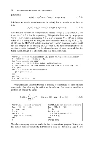
%nm131_1: nested multiplication vs. plain multiple multiplication
N = 1000000+1; a = [1:N]; x = 1;
tic % initialize the timer
p = sum(a.*x.^[N-1:-1:0]); %plain multiplication
p, toc % measure the time passed from the time of executing ’tic’
tic, pn=a(1);
for i = 2:N %nested multiplication
pn = pn*x + a(i);
end
pn, toc
tic, polyval(a,x), toc

Programming in a nested structure is not only recommended for time-efficient
computation, but also may be critical to the solution. For instance, consider a
problem of finding the value

K k
λ −λ
S(K) = e for λ = 100 and K = 155 (1.3.3)
k!
k=0
%nm131_2_1: nested structure %nm131_2_2: not nested structure
lam = 100; K = 155; lam = 100; K = 155;
p = exp(-lam); S=0;
S=0; for k = 1:K
for k = 1:K p = lam^k/factorial(k);
p=p*lam/k; S=S+p; S=S+ p;
end end
S S*exp(-lam)

The above two programs are made for this computational purpose. Noting that
this sum of Poisson probability distribution is close to 1 for such a large K,we