Page 53 - Applied Numerical Methods Using MATLAB

42 MATLAB USAGE AND COMPUTATIONAL ERRORS

1 1

0.5 0.5

0 0

−2 −1 0 1 2 −2 −1 0 1 2
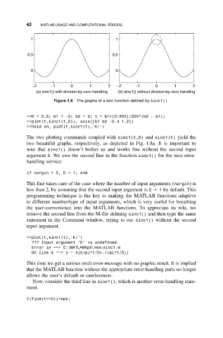
(a) sinc1() with division-by-zero handling (b) sinc1() without division-by-zero handling
Figure 1.8 The graphs of a sinc function defined by sinc1().

>>D = 0.5; b1 = -2; b2 = 2; t = b1+[0:200]/200*(b2 - b1);
>>plot(t,sinc1(t,D)), axis([b1 b2 -0.4 1.2])
>>hold on, plot(t,sinc1(t),’k:’)
The two plotting commands coupled with sinc1(t,D) and sinc1(t) yield the
two beautiful graphs, respectively, as depicted in Fig. 1.8a. It is important to
note that sinc1() doesn’t bother us and works fine without the second input
argument D. We owe the second line in the function sinc1() for the nice error-
handling service:

if nargin < 2,D=1;end

This line takes care of the case where the number of input arguments (nargin)is
less than 2, by assuming that the second input argument is D=1 by default. This
programming technique is the key to making the MATLAB functions adaptive
to different number/type of input arguments, which is very useful for breathing
the user-convenience into the MATLAB functions. To appreciate its role, we
remove the second line from the M-file defining sinc1() and then type the same
statement in the Command window, trying to use sinc1() without the second
input argument.

>>plot(t,sinc1(t),’k:’)
??? Input argument ’D’ is undefined.
Error in ==> C:\MATLAB6p5\nma\sinc1.m
On line 4 ==> x = sin(pi*t/D)./(pi*t/D);
This time we get a serious (red) error message with no graphic result. It is implied
that the MATLAB function without the appropriate error-handling parts no longer
allows the user’s default or carelessness.
Now, consider the third line in sinc1(), which is another error-handling state-
ment.

t(find(t==0))=eps;