Page 56 - Applied Numerical Methods Using MATLAB

TOWARD GOOD PROGRAM 45
functions/routines that are involved with various sets of parameters, you might
find that the global variable is not always convenient, because of the follow-
ing reasons.

ž Once a variable is declared as global, its value can be changed in any of the
MATLAB functions having declared it as global, without being noitced by
other related functions. Therefore it is usual to declare only the constants as
global and use long names (with all capital letters) as their names for easy
identification.
ž If some variables are declared as global and modified by several func-
tions/routines, it is not easy to see the relationship and the interaction among
the related functions in terms of the global variable. In other words, the pro-
gram readability gets worse as the number of global variables and related
functions increases.
For example, let us look over the above program “plot sinc.m” and the func-
tion “sinc2()”. They both have a declaration of D as global; consequently,
sinc2() does not need the second input argument for getting the parameter
D. If you run the program, you will see that the two plotting statements adopting
sinc1() and sinc2() produce the same graphic result as depicted in Fig. 1.8a.

1.3.6 Parameter Passing Through Varargin
In this section we see two kinds of routines that get a function name (string)
with its parameters as its input argument and play with the function.
First, let us look over the routine “ez_plot1()”, which gets a function name
(ftn) with its parameters (p) and the lower/upper bounds (bounds = [b1 b2])
as its first, third, and second input argument, respectively, and plots the graph of
the given function over the interval set by the bounds. Since the given function
may or may not have its parameter, the two cases are determined and processed
by the number of input arguments (nargin)inthe if-else-end block.

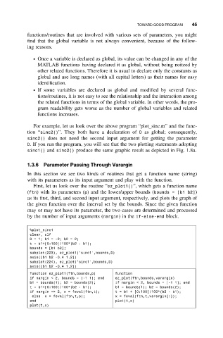
%plot_sinc1
clear, clf
D=1;b1=-2; b2 =2;
t = b1+[0:100]/100*(b2 - b1);
bounds = [b1 b2];
subplot(223), ez_plot1(’sinc1’,bounds,D)
axis([b1 b2 -0.4 1.2])
subplot(224), ez_plot(’sinc1’,bounds,D)
axis([b1 b2 -0.4 1.2])
function ez_plot1(ftn,bounds,p) function
if nargin < 2, bounds = [-1 1]; end ez_plot(ftn,bounds,varargin)
b1 = bounds(1); b2 = bounds(2); if nargin < 2, bounds = [-1 1]; end
t = b1+[0:100]/100*(b2 - b1); b1 = bounds(1); b2 = bounds(2);
if nargin <= 2, x = feval(ftn,t); t = b1 + [0:100]/100*(b2 - b1);
else x = feval(ftn,t,p); x = feval(ftn,t,varargin{:});
end plot(t,x)
plot(t,x)