Page 61 - Applied Numerical Methods Using MATLAB

50 MATLAB USAGE AND COMPUTATIONAL ERRORS
(a) Define the domain vector x consisting of sufficiently many intermediate
point x i ’s along the x-axis and the corresponding vector y consisting
of the function values at x i ’s and plot the vector y over the vector x.
You may use the following statements.
>>x = [0:0.01:2*pi]; y = tan(x);
>>subplot(221), plot(x,y)
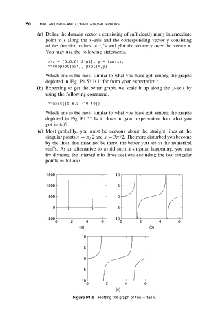
Which one is the most similar to what you have got, among the graphs
depicted in Fig. P1.5? Is it far from your expectation?
(b) Expecting to get the better graph, we scale it up along the y-axis by
using the following command.

>>axis([0 6.3 -10 10])
Which one is the most similar to what you have got, among the graphs
depicted in Fig. P1.5? Is it closer to your expectation than what you
got in (a)?
(c) Most probably, you must be nervous about the straight lines at the
singular points x = π/2and x = 3π/2. The more disturbed you become
by the lines that must not be there, the better you are at the numerical
stuffs. As an alternative to avoid such a singular happening, you can
try dividing the interval into three sections excluding the two singular
points as follows.

1500 10
1000 5

500 0

0 −5

−500 −10
0 2 4 6 0 2 4 6
(a) (b)
10

5

0

−5
−10
0 2 4 6
(c)
Figure P1.5 Plotting the graph of f(x) = tan x.