Page 60 - Applied Numerical Methods Using MATLAB

PROBLEMS 49
(a) At what value of k does MATLAB show you the mesh/surface-type graphs
that are the most similar to the first graphs? From this result, what do you
guess are the default values of the azimuth or horizontal rotation angle and
the vertical elevation angle (in degrees) of the perspective view point?
(b) As the first input argument Az of the command view(Az,E1) decreases,
in which direction does the perspective viewpoint revolve round the
z-axis, clockwise or counterclockwise (seen from the above)?
(c) As the second input argument El of the command view(Az,E1) increases,
does the perspective viewpoint move up or down along the z-axis?
(d) What is the difference between the plotting commands mesh() and
meshc()?
(e) What is the difference between the usages of the command view()
with two input arguments Az,El and with a three-dimensional vector
argument [x,y,z]?

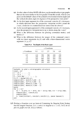
Table P1.4 The Depth of the Rock Layer
x Coordinate
y Coordinate 0.1 1.2 2.5 3.6 4.8

0.5 410 390 380 420 450
1.4 395 375 410 435 455
2.2 365 405 430 455 470
3.5 370 400 420 445 435
4.6 385 395 410 395 410

%nm1p04: to plot a stratigraphic structure
clear, clf
x = [0.1 .. .. . ];
y = [0.5 .. .. . ];
Z = [410 390 .. .. .. .. ];
[X,Y] = meshgrid(x,y);
subplot(221), mesh(X,Y,500 - Z)
subplot(222), surf(X,Y,500 - Z)
subplot(223), meshc(X,Y,500 - Z)
subplot(224), meshz(X,Y,500 - Z)
pause
for k = 0:7
Az = -12.5*k; El = 10*k; Azr = Az*pi/180; Elr = El*pi/180;
subplot(221), view(Az,El)
subplot(222),
k, view([sin(Azr),-cos(Azr),tan(Elr)]), pause %pause(1)
end

1.5 Plotting a Function over an Interval Containing Its Singular Point Noting
that the tangent function f(x) = tan(x) is singular at x = π/2, 3π/2, let us
plot its graph over [0, 2π] as follows.