Page 64 - Applied Numerical Methods Using MATLAB

PROBLEMS 53
where

1 −(x−m) /2σ 2
2
x 0 = 1, f (x) = √ e with m = 1,σ = 2 (P1.8.3)
2πσ
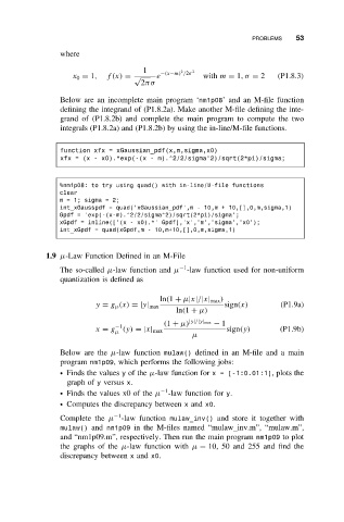
Below are an incomplete main program ‘nm1p08’ and an M-file function
defining the integrand of (P1.8.2a). Make another M-file defining the inte-
grand of (P1.8.2b) and complete the main program to compute the two
integrals (P1.8.2a) and (P1.8.2b) by using the in-line/M-file functions.

function xfx = xGaussian_pdf(x,m,sigma,x0)
xfx = (x - x0).*exp(-(x - m).^2/2/sigma^2)/sqrt(2*pi)/sigma;

%nm1p08: to try using quad() with in-line/M-file functions
clear
m = 1; sigma = 2;
int_xGausspdf = quad(’xGaussian_pdf’,m - 10,m + 10,[],0,m,sigma,1)
Gpdf = ’exp(-(x-m).^2/2/sigma^2)/sqrt(2*pi)/sigma’;
xGpdf = inline([’(x - x0).*’ Gpdf],’x’,’m’,’sigma’,’x0’);
int_xGpdf = quad(xGpdf,m - 10,m+10,[],0,m,sigma,1)

1.9 µ-Law Function Defined in an M-File
−1
The so-called µ-law function and µ -law function used for non-uniform
quantization is defined as

ln(1 + µ|x|/|x| max )
y = g µ (x) =|y| max sign(x) (P1.9a)
ln(1 + µ)
(1 + µ) |y|/|y| max − 1
−1
x = g (y) =|x| max sign(y) (P1.9b)
µ
µ
Below are the µ-law function mulaw() defined in an M-file and a main
program nm1p09, which performs the following jobs:
ž Finds the values y of the µ-law function for x = [-1:0.01:1], plots the
graph of y versus x.
−1
ž Finds the values x0 of the µ -law function for y.
ž Computes the discrepancy between x and x0.
−1
Complete the µ -law function mulaw_inv() and store it together with
mulaw() and nm1p09 in the M-files named “mulaw inv.m”, “mulaw.m”,
and “nm1p09.m”, respectively. Then run the main program nm1p09 to plot
the graphs of the µ-law function with µ = 10, 50 and 255 and find the
discrepancy between x and x0.