Page 48 - Applied Numerical Methods Using MATLAB

TOWARD GOOD PROGRAM 37

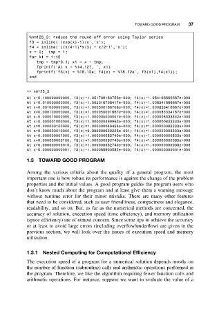
%nm125_3: reduce the round-off error using Taylor series
f3 = inline(’(exp(x)-1)/x’,’x’);
f4 = inline(’((x/4+1)*x/3) + x/2+1’,’x’);
x=0; tmp=1;
for k1 = 1:12
tmp = tmp*0.1; x1 = x + tmp;
fprintf(’At x = %14.12f, ’, x1)
fprintf(’f3(x) = %18.12e; f4(x) = %18.12e’, f3(x1),f4(x1));
end

>> nm125_3
At x=0.100000000000, f3(x)=1.051709180756e+000; f4(x)=1.084166666667e+000
At x=0.010000000000, f3(x)=1.005016708417e+000; f4(x)=1.008341666667e+000
At x=0.001000000000, f3(x)=1.000500166708e+000; f4(x)=1.000833416667e+000
At x=0.000100000000, f3(x)=1.000050001667e+000; f4(x)=1.000083334167e+000
At x=0.000010000000, f3(x)=1.000005000007e+000; f4(x)=1.000008333342e+000
At x=0.000001000000, f3(x)=1.000000499962e+000; f4(x)=1.000000833333e+000
At x=0.000000100000, f3(x)=1.000000049434e+000; f4(x)=1.000000083333e+000
At x=0.000000010000, f3(x)=9.999999939225e-001; f4(x)=1.000000008333e+000
At x=0.000000001000, f3(x)=1.000000082740e+000; f4(x)=1.000000000833e+000
At x=0.000000000100, f3(x)=1.000000082740e+000; f4(x)=1.000000000083e+000
At x=0.000000000010, f3(x)=1.000000082740e+000; f4(x)=1.000000000008e+000
At x=0.000000000001, f3(x)=1.000088900582e+000; f4(x)=1.000000000001e+000

1.3 TOWARD GOOD PROGRAM

Among the various criteria about the quality of a general program, the most
important one is how robust its performance is against the change of the problem
properties and the initial values. A good program guides the program users who
don’t know much about the program and at least give them a warning message
without runtime error for their minor mistake. There are many other features
that need to be considered, such as user friendliness, compactness and elegance,
readability, and so on. But, as far as the numerical methods are concerned, the
accuracy of solution, execution speed (time efficiency), and memory utilization
(space efficiency) are of utmost concern. Since some tips to achieve the accuracy
or at least to avoid large errors (including overflow/underflow) are given in the
previous section, we will look over the issues of execution speed and memory
utilization.

1.3.1 Nested Computing for Computational Efficiency
The execution speed of a program for a numerical solution depends mostly on
the number of function (subroutine) calls and arithmetic operations performed in
the program. Therefore, we like the algorithm requiring fewer function calls and
arithmetic operations. For instance, suppose we want to evaluate the value of a