Page 174 - Applied Petroleum Geomechanics

168 Applied Petroleum Geomechanics

120

110
100 RF
(MPa) 90 SS

σH
80 σv
NF
70
σ σv = 82.5 MPa
Pp = 69.7 MPa
60
60 70 80 90 100 110 120
σh (MPa)
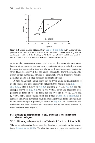
Figure 5.3 Stress polygon obtained from Eqs. (5.11) and (5.12) with measured pore
pressure of 69.7 MPa and vertical stress of 82.5 MPa in a borehole, assuming that the
coefficient of friction of the fault (m f ) is 0.6. In the plot, NF, SS, and RF represent the
normal, strike-slip, and reverse faulting stress regimes, respectively.

stress to the overburden stress. However, in the strike-slip and thrust
faulting stress regimes, the maximum horizontal stress should be located
between the overburden stress and the upper bound maximum horizontal
stress. It can be observed that the range between the lower bound and the
upper bound horizontal stresses is significant, which therefore requires
dedicated efforts to better constrain horizontal stresses.
A stress polygon at a given depth can be drawn using the relationships of
in situ stresses and pore pressure in different stress regimes from Eqs. (5.11)
and (5.12). This is shown in Fig. 5.3 assuming m f ¼ 0.6. Fig. 5.3 uses the
example shown in Fig. 5.2, where the vertical stress and measured pore
pressure at depth of 4316 m from the sea level are s V ¼ 82.5 MPa and
p p ¼ 69.7 MPa. Biot’s coefficient of 1 is applied to Eqs. (5.11) and (5.12) to
calculate the lower and upper bound horizontal stresses. From these data, an
in situ stress polygon is plotted, as shown in Fig. 5.3. The maximum and
minimum horizontal stresses are constrained inside the stress polygon in
three different stress regimes.

5.3 Lithology-dependent in situ stresses and improved
stress polygon
5.3.1 Lithology-dependent coefficient of friction of the fault
The stress polygon has been used for decades to constrain in situ stresses
(e.g., Zoback et al., 2003). To plot the stress polygon, the coefficient of