Page 194 - Applied Petroleum Geomechanics

In situ stress estimate 189

based on analyzing the observed depthedensity curve in density measure-
ments of shales in northern Oklahoma. It has the following relation:
r ¼ r þ A m ð1 e bZ Þ (6.3)
z
0
3
where r z is the density at the depth of Z, in g/cm ; r 0 is the formation
density at the surface; A m is the possible maximum density increase
(A m ¼ r m r 0 and A m ¼ 1.3 in Athy (1930)); r m is the matrix density or
the grain density of the rock; b is a fitting constant. When bulk density
data (r z ) are available at certain depths, by fitting the density curve to
Eq. (6.3), the shallow density (r 0 ) can be obtained.
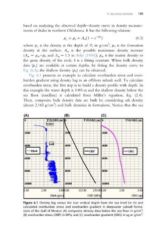
Fig. 6.1 presents an example to calculate overburden stress and over-
burden gradient using density log in an offshore subsalt well. To calculate
overburden stress, the first step is to build a density profile with depth. In
this example the water depth is 1085 m and the shallow density below the
sea floor (mudline) is calculated from Miller’s equation, Eq. (2.4).
Then, composite bulk density data are built by considering salt density
3
(about 2.165 g/cm ) and bulk densities in formations. Notice that the sea

Figure 6.1 Density log versus the true vertical depth from the sea level (in m) and
calculated overburden stress and overburden gradient in deepwater subsalt forma-
3
tions of the Gulf of Mexico: (A) composite density data below the sea floor in g/cm ;
3
(B) overburden stress (OBP) in MPa; and (C) overburden gradient (OBG) in sg or g/cm .