Page 205 - Applied Probability

9. Descent Graph Methods
190
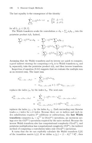
The last equality is the consequence of the identity

0 j r = l r
k r =0
for all l r ,j r ∈{0, 1}. 1 (−1) k r (l r −j r ) = , 2 j r = l r

The Walsh transform sends the convolution a ∗ b k = a j b k−j into the
j
ˆ
pointwise product ˆ a l b l . Indeed,

(−1) l,k a ∗ b k = (−1) l,k a j b k−j
k k j

= (−1) l,j a j (−1) l,k−j b k−j
j k

= (−1) l,j a j (−1) l,j b j .
j j
Assuming that the Walsh transform and its inverse are quick to compute,
a good indirect strategy for computing a ∗ b k is to Walsh transform a k and
ˆ
b k separately, take the pointwise product ˆ a l b l , and then inverse transform.
Inspection of equation (9.14) suggests that we evaluate the multiple sum
as an iterated sum. The inner sum
1
(1)
a = (−1) k m j m a j
(j 1 ,...,j m−1 ,k m )
j m =0
= a (j 1 ,...,j m−1 ,0) +(−1) k m a (j 1 ,...,j m−1 ,1) .
replaces the index j m by the index k m . The next sum
1
(2) (1)
a = (−1) k m−1 j m−1 a
(j 1 ,...,j m−2 ,k m−1 ,k m ) (j 1 ,...,j m−2 ,j m−1 ,k m )
j m−1 =0
(1) (1)
= a +(−1) k m−1 a
(j 1 ,...,j m−2 ,0,k m ) (j 1 ,...,j m−2 ,1,k m )
replaces the index j m−1 by the index k m−1 . Each succeeding sum likewise
trades a j index for a k index. Because there are m indices and each in-
dex substitution requires 2 m additions or subtractions, this fast Walsh
(m) m
transform computes ˆ a k = a k in O(m2 ) operations, an enormous sav-
ings over the O(2 2m ) operations required by the naive method. Because the
m
inverse Walsh transform also has computational complexity O(m2 ), and
m
pointwise multiplication has computational complexity O(2 ), the indirect
m
method of computing a convolution takes only O(m2 ) operations.
It turns that the we can explicitly calculate the Walsh transform ˆ t i (k)
j r
of the transition matrix t i (j). If we define s r (j r )=(1 − θ i ) 1−j r θ , then
i