Page 196 - Applied Statistics And Probability For Engineers

c05.qxd 5/13/02 1:50 PM Page 172 RK UL 6 RK UL 6:Desktop Folder:TEMP WORK:MONTGOMERY:REVISES UPLO D CH114 FIN L:Quark Files:

172 CHAPTER 5 JOINT PROBABILITY DISTRIBUTIONS

Definition
h1x, y2 f 1x, y2 X, Y discrete
b XY
R
E3h1X, Y24 µ (5-27)
h1x, y2 f 1x, y2 dx dy X, Y continuous
XY
R

That is, E[h(X, Y)] can be thought of as the weighted average of h(x, y) for each point in the
range of (X,Y). The value of E[h(X,Y)] represents the average value of h(X,Y) that is expected
in a long sequence of repeated trials of the random experiment.

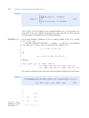
EXAMPLE 5-27 For the joint probability distribution of the two random variables in Fig. 5-12, calculate
E31X 2 1Y 24.
X
Y
The result is obtained by multiplying x times y , times f (x, y) for each point
X
XY
Y
in the range of (X, Y). First, and are determined from Equation 5-3 as
Y
X
1 0.3 3 0.7 2.4
X
and
1 0.3 2 0.4 3 0.3 2.0
Y
Therefore,

E31X 21Y 24 11 2.4211 2.02 0.1
Y
X
11 2.4212 2.02 0.2 13 2.4211 2.02 0.2
13 2.4212 2.02 0.2 13 2.4213 2.02 0.3 0.2
The covariance is defined for both continuous and discrete random variables by the same formula.

Definition
The covariance between the random variables X and Y, denoted as cov(X, Y) or XY , is

E31X 21Y 24 E1XY2 (5-28)
XY X Y X Y

y

3 0.3

2 0.2 0.2

1 0.1 0.2
Figure 5-12 Joint
distribution of X and Y
for Example 5-27. 1 2 3 x