Page 199 - Applied Statistics And Probability For Engineers

c05.qxd 5/13/02 1:50 PM Page 175 RK UL 6 RK UL 6:Desktop Folder:TEMP WORK:MONTGOMERY:REVISES UPLO D CH114 FIN L:Quark Files:

5-5 COVARIANCE AND CORRELATION 175

If the points in the joint probability distribution of X and Y that receive positive probabil-
ity tend to fall along a line of positive (or negative) slope, XY is near 1 (or 1). If XY
equals 1 or 1, it can be shown that the points in the joint probability distribution that
receive positive probability fall exactly along a straight line. Two random variables with
nonzero correlation are said to be correlated. Similar to covariance, the correlation is a meas-
ure of the linear relationship between random variables.

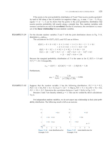
EXAMPLE 5-29 For the discrete random variables X and Y with the joint distribution shown in Fig. 5-14,
determine XY and XY .
The calculations for E(XY), E(X), and V(X) are as follows.

E1XY 2 0 0 0.2 1 1 0.1 1 2 0.1 2 1 0.1
2 2 0.1 3 3 0.4 4.5
E1X2 0 0.2 1 0.2 2 0.2 3 0.4 1.8
2
2
2
V1X 2 10 1.82 0.2 11 1.82 0.2 12 1.82 0.2
2
13 1.82 0.4 1.36
Because the marginal probability distribution of Y is the same as for X, E(Y) 1.8 and
V(Y) 1.36. Consequently,
E1XY2 E1X2E1Y2 4.5 11.8211.82 1.26
XY
Furthermore,

XY 1.26
0.926
Y 1 11.3621 11.362
XY
X
EXAMPLE 5-30 Suppose that the random variable X has the following distribution: P(X 1) 0.2,
P(X 2) 0.6, P(X 3) 0.2. Let Y 2X 5. That is, P(Y 7) 0.2, P(Y 9) 0.6,
P(Y 11) 0.2. Determine the correlation between X and Y. Refer to Fig. 5-15.
Because X and Y are linearly related, 1. This can be verified by direct calculations:
Try it.

For independent random variables, we do not expect any relationship in their joint prob-
ability distribution. The following result is left as an exercise.

y y
3 0.4 11 0.2

2 0.1 0.1 9 0.6

1 0.1 0.1 7 0.2
ρ = 1
0.2
0
0 1 2 3 x 1 2 3 x
Figure 5-14 Joint distribution for Figure 5-15 Joint distribution for
Example 5-29. Example 5-30.