Page 202 - Applied Statistics And Probability For Engineers

c05.qxd 5/13/02 1:50 PM Page 178 RK UL 6 RK UL 6:Desktop Folder:TEMP WORK:MONTGOMERY:REVISES UPLO D CH114 FIN L:Quark Files:

178 CHAPTER 5 JOINT PROBABILITY DISTRIBUTIONS

chapter, if the specifications for X and Y are 2.95 to 3.05 and 7.60 to 7.80 millimeters, respec-
tively, we might be interested in the probability that a part satisfies both specifications; that is,
P(2.95 X 3.05, 7.60 Y 7.80).

Definition
The probability density function of a bivariate normal distribution is

2
1 1 1x 2
X
f 1x, y; , , , , 2 exp e c
XY X Y X Y 2 2 2
2 21 211 2 X
X Y
2
2 1x 21y 2 1y 2
X
Y
Y
X Y Y 2 df (5-32)
for
x
and
y
, with parameters X
0,
0,

,
X
Y

, and 1 1.
Y
The result that f XY (x, y; X , Y , X , Y , ) integrates to 1 is left as an exercise. Also, the bivari-
ate normal probability density function is positive over the entire plane of real numbers.
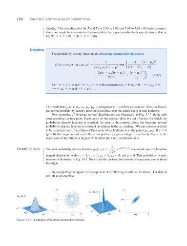
Two examples of bivariate normal distributions are illustrated in Fig. 5-17 along with
corresponding contour plots. Each curve on the contour plots is a set of points for which the
probability density function is constant. As seen in the contour plots, the bivariate normal
probability density function is constant on ellipses in the (x, y) plane. (We can consider a circle
to be a special case of an ellipse.) The center of each ellipse is at the point ( X , Y ). If
0
( 0), the major axis of each ellipse has positive (negative) slope, respectively. If 0, the
major axis of the ellipse is aligned with either the x or y coordinate axis.

1 2 2
EXAMPLE 5-33 The joint probability density function f XY 1x, y2 e 0.51x y 2 is a special case of a bivariate
12
normal distribution with X 1, Y 1, X 0, Y 0, and 0. This probability density
function is illustrated in Fig. 5-18. Notice that the contour plot consists of concentric circles about
the origin.

By completing the square in the exponent, the following results can be shown. The details
are left as an exercise.

y y
f XY (x, y)
(x, y)
f f XY (x, y)
XY
Y Y
y
y
Y x Y x
X X x X X x
0
Figure 5-17 Examples of bivariate normal distributions.