Page 214 - Applied Statistics And Probability For Engineers

PQ220 6234F.CD(05) 5/13/02 4:51 PM Page 2 RK UL 6 RK UL 6:Desktop Folder:TEMP WORK:MONTGOMERY:REVISES UPLO D CH114 FIN L:Quark F

5-2

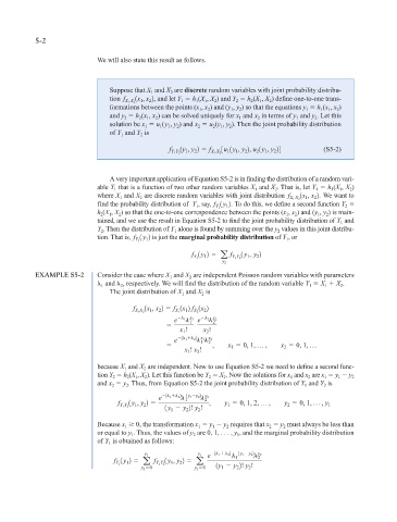
We will also state this result as follows.

Suppose that X and X are discrete random variables with joint probability distribu-
2
1
1x , x 2, h (X , X ) and Y h (X , X ) define one-to-one trans-
tion f X 1 X 2 1 2 and let Y 1 1 1 2 2 2 1 2
formations between the points (x , x ) and (y , y ) so that the equations y h (x , x )
2
2
1
1
2
1
1
1
and y h (x , x ) can be solved uniquely for x and x in terms of y and y . Let this
2
2
2
1
2
1
2
1
solution be x u (y , y ) and x u (y , y ). Then the joint probability distribution
2
2
2
1
1
1
2
1
of Y and Y is
1
2
f 1y , y 2 f 3u 1y , y 2, u 1y , y 24 (S5-2)
2
1
1
2
1
2
1
2
Y 1 Y 2 X 1 X 2
A very important application of Equation S5-2 is in finding the distribution of a random vari-
able Y that is a function of two other random variables X and X . That is, let Y h (X , X )
1
1
2
1
1
2
1
where X and X are discrete random variables with joint distribution f X 1 X 2 1 2 We want to
1x , x 2.
1
2
, say, f 1 y 2. To do this, we define a second function Y
find the probability distribution of Y 1 1 2
Y 1
h (X , X ) so that the one-to-one correspondence between the points (x , x ) and (y , y ) is main-
1
1
1
2
2
2
2
tained, and we use the result in Equation S5-2 to find the joint probability distribution of Y and
1
Y . Then the distribution of Y alone is found by summing over the y values in this joint distribu-
1
2
2
tion. That is, f 1y 2 is just the marginal probability distribution of Y , or
1
Y 1 1
f 1 y 2 f 1y , y 2
Y 1 1 a Y 1 Y 2 1 2
y 2
EXAMPLE S5-2 Consider the case where X and X are independent Poisson random variables with parameters
2
1
and , respectively. We will find the distribution of the random variable Y X X .
1
2
2
1
1
The joint distribution of X and X is
2
1
f 1x , x 2 f 1x 2 f 1x 2
1
2
1
2
X 1 X 2 X 1 X 2

e 1 x 1 e 2 x 2
2
1

x ! x !
2
1

e 1 1 2 2 x 1 x 2
1
2
, x 0, 1, p , x 0, 1, p
1
2
x ! x !
1
2
because X and X are independent. Now to use Equation S5-2 we need to define a second func-
1
2
tion Y h (X , X ). Let this function be Y X . Now the solutions for x and x are x y y 2
1
2
2
1
2
2
1
1
2
2
and x y . Thus, from Equation S5-2 the joint probability distribution of Y and Y is
2
2
1
2

e 1 1 2 2 1 1 y 1 y 2 2 y 2
2
1 y , y 2 , y 0, 1, 2, p , y 0, 1, p , y
1 y 1 y 2 2! y 2 !
f Y 1 Y 2 1 2 1 2 1
Because x 0, the transformation x y y requires that x y must always be less than
1
1
1
2
2
2
or equal to y . Thus, the values of y are 0, 1, . . . , y , and the marginal probability distribution
1
1
2
of Y is obtained as follows:
1

y 1 y 1 e 1 1 2 2 1 y 1 y 2 2 y 2
1 y 2 a f 1 y , y 2 a 1 2
f Y 1 1 Y 1 Y 2 1 2
2
1
2
y 2 0 y 2 0 1y y 2! y !