Page 310 - Applied Statistics And Probability For Engineers

c08.qxd 5/15/02 6:13 PM Page 262 RK UL 6 RK UL 6:Desktop Folder:TEMP WORK:MONTGOMERY:REVISES UPLO D CH114 FIN L:Quark Files:

262 CHAPTER 8 STATISTICAL INTERVALS FOR A SINGLE SAMPLE

Definition
Let X , X , p , X be a random sample from a normal distribution with mean and
1
n
2
2
2
variance , and let S be the sample variance. Then the random variable
1n 12 S 2
2
X (8-19)
2
2
has a chi-square ( ) distribution with n 1 degrees of freedom.
2
The probability density function of a random variable is
1
f 1x2 x 1k 22 1 x 2 x
0 (8-20)
e
2 1k 22
k 2
2
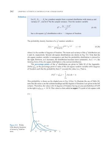
where k is the number of degrees of freedom. The mean and variance of the distribution are
k and 2k, respectively. Several chi-square distributions are shown in Fig. 8-8. Note that the
chi-square random variable is nonnegative and that the probability distribution is skewed to
the right. However, as k increases, the distribution becomes more symmetric. As k S
, the
limiting form of the chi-square distribution is the normal distribution.
2
The percentage points of the distribution are given in Table III of the Appendix.
2
Define ,k as the percentage point or value of the chi-square random variable with k degrees
2
of freedom such that the probability that X exceeds this value is . That is,

2
2
P1X
,k 2 f 1u2 du
2
,k
This probability is shown as the shaded area in Fig. 8-9(a). To illustrate the use of Table III,
note that the areas are the column headings and the degrees of freedom k are given in the left
column. Therefore, the value with 10 degrees of freedom having an area (probability) of 0.05
2
to the right is 0.05,10 18.31. This value is often called an upper 5% point of chi-square with
f (x)

k = 2

k = 5
Figure 8-8 Proba-
k = 10
bility density functions
2
of several distribu-
tions. 0 5 10 15 20 25 x