Page 306 - Applied Statistics And Probability For Engineers

c08.qxd 5/15/02 6:13 PM Page 258 RK UL 6 RK UL 6:Desktop Folder:TEMP WORK:MONTGOMERY:REVISES UPLO D CH114 FIN L:Quark Files:

258 CHAPTER 8 STATISTICAL INTERVALS FOR A SINGLE SAMPLE

Section 8-2.5. However, n is usually small in most engineering problems, and in this situation
a different distribution must be employed to construct the CI.

8-3.1 The t Distribution

Definition
Let X , X , p , X be a random sample from a normal distribution with unknown
2
n
1
2
mean and unknown variance . The random variable
X
T (8-15)
S 1n
has a t distribution with n 1 degrees of freedom.

The t probability density function is

31k 12 24 1
f 1x2 2 1k 12 2
x
(8-16)
2 k 1k 22 31x k2 14
where k is the number of degrees of freedom. The mean and variance of the t distribution are
zero and k/(k 2) (for k
2), respectively.
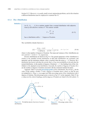
Several t distributions are shown in Fig. 8-4. The general appearance of the t distribution is
similar to the standard normal distribution in that both distributions are symmetric and
unimodal, and the maximum ordinate value is reached when the mean 0. However, the t
distribution has heavier tails than the normal; that is, it has more probability in the tails than the
normal distribution. As the number of degrees of freedom k S
, the limiting form of the t dis-
tribution is the standard normal distribution. Generally, the number of degrees of freedom for t
are the number of degrees of freedom associated with the estimated standard deviation.
be the
Appendix Table IV provides percentage points of the t distribution. We will let t ,k
value of the random variable T with k degrees of freedom above which we find an area
(or probability) . Thus, t ,k is an upper-tail 100 percentage point of the t distribution with k
degrees of freedom. This percentage point is shown in Fig. 8-5. In the Appendix Table IV the
values are the column headings, and the degrees of freedom are listed in the left column. To

k = 10

k = ∞ [N (0, 1)]

k = 1

α α

0 x t 1 – α, k = – t α, k 0 t α, k t
Figure 8-4 Probability density functions of several t Figure 8-5 Percentage points of the t
distributions. distribution.