Page 308 - Applied Statistics And Probability For Engineers

c08.qxd 5/16/02 12:54 PM Page 260 RK UL 6 RK UL 6:Desktop Folder:TEMP WORK:MONTGOMERY:REVISES UPLO D CH 1 14 FIN L:Quark Files:

260 CHAPTER 8 STATISTICAL INTERVALS FOR A SINGLE SAMPLE

Normal probability plot
99
95
20.5 90
80
18.0 Percent 70
Load at failure 15.5 40
60
50
30
20
13.0
10.5 10 5
1
8.0 5 10 15 20 25
Load at failure
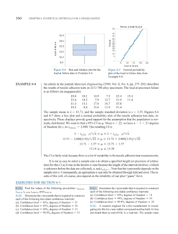
Figure 8-6 Box and whisker plot for the Figure 8-7 Normal probability
load at failure data in Example 8-4. plot of the load at failure data from
Example 8-4.

EXAMPLE 8-4 An article in the journal Materials Engineering (1989, Vol. II, No. 4, pp. 275–281) describes
the results of tensile adhesion tests on 22 U-700 alloy specimens. The load at specimen failure
is as follows (in megapascals):
19.8 10.1 14.9 7.5 15.4 15.4
15.4 18.5 7.9 12.7 11.9 11.4
11.4 14.1 17.6 16.7 15.8
19.5 8.8 13.6 11.9 11.4
The sample mean is 13.71, and the sample standard deviation is s 3.55. Figures 8-6
x
and 8-7 show a box plot and a normal probability plot of the tensile adhesion test data, re-
spectively. These displays provide good support for the assumption that the population is nor-
mally distributed. We want to find a 95% CI on . Since n 22, we have n 1 21 degrees
of freedom for t, so t 0.025,21 2.080. The resulting CI is

x t 2,n 1 s 1n x t 2,n 1 s 1n
13.71 2.08013.552 122 13.71 2.08013.552 122
13.71 1.57 13.71 1.57
12.14 15.28
The CI is fairly wide because there is a lot of variability in the tensile adhesion test measurements.

It is not as easy to select a sample size n to obtain a specified length (or precision of estima-
tion) for this CI as it was in the known- case because the length of the interval involves s (which
. Note that the t-percentile depends on the
is unknown before the data are collected), n, and t 2,n 1
sample size n. Consequently, an appropriate n can only be obtained through trial and error. The re-
sults of this will, of course, also depend on the reliability of our prior “guess” for .
EXERCISES FOR SECTION 8-3

8-19. Find the values of the following percentiles: t 0.025,15 , 8-21. Determine the t-percentile that is required to construct
t 0.05,10 , t 0.10,20 , t 0.005,25 , and t 0.001,30 . each of the following one-sided confidence intervals:
8-20. Determine the t-percentile that is required to construct (a) Confidence level 95%, degrees of freedom 14
each of the following two-sided confidence intervals: (b) Confidence level 99%, degrees of freedom 19
(a) Confidence level 95%, degrees of freedom 12 (c) Confidence level 99.9%, degrees of freedom 24
(b) Confidence level 95%, degrees of freedom 24 8-22. A research engineer for a tire manufacturer is investi-
(c) Confidence level 99%, degrees of freedom 13 gating tire life for a new rubber compound and has built 16 tires
(d) Confidence level 99.9%, degrees of freedom 15 and tested them to end-of-life in a road test. The sample mean