Page 131 - Applied statistics and probability for engineers

Section 4-2/Probability Distributions and Probability Density Functions 109

Similarly, a probability density function f x ( ) can be used to describe the probability
distribution of a continuous random variable X. If an interval is likely to contain a value for X,
its probability is large and it corresponds to large values for f x ( ). The probability that X is
between a and b is determined as the integral of f x ( ) from a to b. See Fig. 4-2.

Probability Density
Function For a continuous random variable X, a probability density function is a function
such that
(1) f x ( ) ≥ 0
∞
(2) ∫ f x dx = 1
(
)
−∞
( )
(3) ( X ≤ b) = b ∫ f x dx = area under f x ( ) from a to b for any a and b (4-1)
P a ≤
a
A probability density function provides a simple description of the probabilities associated
with a random variable. As long as f x ( ) is nonnegative and −∞ ∫ ∞ f x ( ) = 1 , 0 ≤ (a , X , b ) ≤ 1
P
so that the probabilities are properly restricted. A probability density function is zero for x
values that cannot occur, and it is assumed to be zero wherever it is not speciically deined.
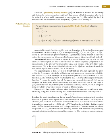
A histogram is an approximation to a probability density function. See Fig. 4-3. For each
interval of the histogram, the area of the bar equals the relative frequency (proportion) of the
measurements in the interval. The relative frequency is an estimate of the probability that a
measurement falls in the interval. Similarly, the area under f x ( ) over any interval equals the
true probability that a measurement falls in the interval.
The important point is that f x ( ) is used to calculate an area that represents the prob-
ability that X assumes a value in [a, b]. For the current measurement example, the probability
that X results in [14 mA, 15 mA] is the integral of the probability density function of X over
this interval. The probability that X results in [14.5 mA, 14.6 mA] is the integral of the same
function, f x ( ), over the smaller interval. By appropriate choice of the shape of f x ( ), we can
represent the probabilities associated with any continuous random variable X. The shape of
f x ( ) determines how the probability that X assumes a value in [14.5 mA, 14.6 mA] compares
to the probability of any other interval of equal or different length.
For the density function of a loading on a long, thin beam, because every point has zero width,
the loading at any point is zero. Similarly, for a continuous random variable X and any value x,
(
P X = x) = 0
Based on this result, it might appear that our model of a continuous random variable is useless.
However, in practice, when a particular current measurement such as 14.47 milliamperes, is
observed, this result can be interpreted as the rounded value of a current measurement that
is actually in a range such as 14 465 ≤ ≤ 14 475. Therefore, the probability that the rounded
.
.
x
value 14.47 is observed as the value for X is the probability that X assumes a value in the inter-
val [14.465, 14.475], which is not zero. Similarly, because each point has zero probability,
one need not distinguish between inequalities such as < or ≤ for continuous random variables.
f(x)

x
FIGURE 4-3 Histogram approximates a probability density function.