Page 134 - Applied statistics and probability for engineers

112 Chapter 4/Continuous Random Variables and Probability Distributions

4-3 Cumulative Distribution Functions

An alternative method to describe the distribution of a discrete random variable can also be
used for continuous random variables.

Cumulative
Distribution Function The cumulative distribution function of a continuous random variable X is

( )
P X ≤
F x ( ) = ( x) = x ∫ f u du (4-3)
for −∞ < x < ∞. −∞

The cumulative distribution function is deined for all real numbers. The following example

illustrates the dei nition.

Example 4-3 Electric Current For the copper current measurement in Example 4-1, the cumulative
distribution function of the random variable X consists of three expressions. If x < 4 9 ( 0.

, f x) =
.
Therefore,
F x ( ) = 0 , for x < 4.9
and
x
( )
F x ( ) = ∫ f u du = 5 x − 24 5. , for 4 9 ≤ x < 5 1
.
.
.
4 9
Finally,
x
( )
F x ( ) = ∫ f u du = 1 , for 5 1 ≤ x
.
4 9
.
Therefore,
.
⎧0 x < 4 9
⎪
.
.
F x ( ) = ⎨ 5 x − 24 5 4 9 ≤ x < 5 1
.
⎪ ≤
.
⎩ 1 5 1 x
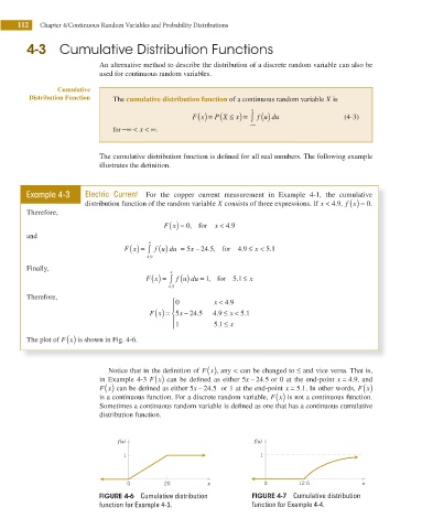
The plot of F x ( ) is shown in Fig. 4-6.
Notice that in the dei nition of F x ( ), any < can be changed to ≤ and vice versa. That is,
in Example 4-3 F x ( ) can be dei ned as either 5 − 24 5 or 0 at the end-point x = 4 9 , and
x
.
.
.
.
F x ( ) can be deined as either 5x − 24 5 or 1 at the end-point x = 5 1 . In other words, F x ( )

is a continuous function. For a discrete random variable, F x ( ) is not a continuous function.
Sometimes a continuous random variable is deined as one that has a continuous cumulative

distribution function.
f(x) f(x)
1 1
0 20 x 0 12.5 x
FIGURE 4-6 Cumulative distribution FIGURE 4-7 Cumulative distribution
function for Example 4-3. function for Example 4-4.