Page 137 - Applied statistics and probability for engineers

Section 4-4/Mean and Variance of a Continuous Random Variable 115

The equivalence of the two formulas for variance can be derived from the same approach used
for discrete random variables.

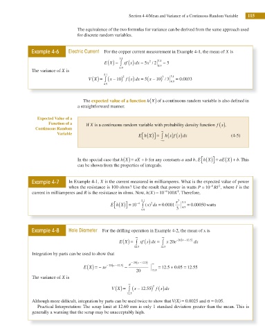
Example 4-6 Electric Current For the copper current measurement in Example 4-1, the mean of X is

5 1 .
( )
E X ( ) = ∫ xf x dx = 5 x / 2 5 1 . = 5
2
4 9 . 4 9 .
The variance of X is
5 1 .
.
3
2
V X ( ) = ( ∫ x − ) ( ) x − ) 3 / 5 1 = 0.0033
10
f x dx = ( 5
10
4 9
.
4 9 .
The expected value of a function h X ( ) of a continuous random variable is also dei ned in
a straightforward manner.
Expected Value of a
Function of a If X is a continuous random variable with probability density function f x ( ),
Continuous Random
( ) (
Variable ∞ h x f x dx )
⎡
E h X ( )⎤ = ∫ (4-5)
⎣
⎦
−∞
⎡
In the special case that h X ( ) = aX + b for any constants a and b, E h X ( )⎤ = aE X ( ) + b. This
⎦
⎣
can be shown from the properties of integrals.
Example 4-7 In Example 4-1, X is the current measured in milliamperes. What is the expected value of power
2
when the resistance is 100 ohms? Use the result that power in watts P = 10 −6 RI , where I is the
−
6
2
current in milliamperes and R is the resistance in ohms. Now, h X) = 10 100 X . Therefore,
(
5 1 . x 3 5 1 .
⎡
E h X ( )⎤ = 10 −4 ∫ ( ) 2 . = 0 00050watts
x dx = 0 0001
.
⎣
⎦
4 9 . 3 4 9 .
Example 4-8 Hole Diameter For the drilling operation in Example 4-2, the mean of x is
∞ ∞ − ( )
( )
E X ( ) = ∫ xf x dx = ∫ x 20 e 20 x − 12 5. dx
.
.
12 5 12 5
Integration by parts can be used to show that
− ( x − 12 5 . ) ∞
20
e
E X ( ) = − xe − ( x − 12 5 . ) − = 12 5. + 0 05. = 12 55.
20
20 12 5 .
The variance of X is
∞
f x dx )
2
V X ( ) = ( ∫ x − 12 55 ) (
.
.
12 5

Although more dificult, integration by parts can be used twice to show that V(X) = 0.0025 and σ = 0.05.
Practical Interpretation: The scrap limit at 12.60 mm is only 1 standard deviation greater than the mean. This is
generally a warning that the scrap may be unacceptably high.