Page 142 - Applied statistics and probability for engineers

120 Chapter 4/Continuous Random Variables and Probability Distributions

f (x) s 2 = 1 f (x)
s 2 = 1
s 2 = 4

m = 5 m = 15 x
10 13 x
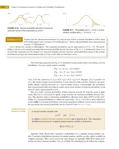
FIGURE 4-10 Normal probability density functions for
2
selected values of the parameters μ and σ . FIGURE 4-11 Probability that X > 13 for a normal
random variable with μ = 10 and σ = .
2
4
Example 4-10 Assume that the current measurements in a strip of wire follow a normal distribution with a mean
2
of 10 milliamperes and a variance of 4 (milliamperes) . What is the probability that a measurement
exceeds 13 milliamperes?
(
Let X denote the current in milliamperes. The requested probability can be represented as P X > 13). This prob-
ability is shown as the shaded area under the normal probability density function in Fig. 4-11. Unfortunately, there is no
closed-form expression for the integral of a normal probability density function, and probabilities based on the normal
distribution are typically found numerically or from a table (that we introduce soon).

The following equations and Fig. 4-12 summarize some useful results concerning a normal
distribution. For any normal random variable,
(
.
P μ − s < X < μ + ) =s 0 6827
(
P μ − 2s < X < μ + ) = 0 9545
s
2
.
(
P μ − 3s < X < μ + ) = 0 9973
.
s
3
( )
Also, from the symmetry of f x ,P X ( < μ) = P X ( < μ) = . . Because f x ( ) is positive for
0
5
all x, this model assigns some probability to each interval of the real line. However, the prob-
ability density function decreases as x moves farther from μ. Consequently, the probability
that a measurement falls far from μ is small, and at some distance from μ, the probability of an
interval can be approximated as zero.
The area under a normal probability density function beyond 3σ from the mean is quite
small. This fact is convenient for quick, rough sketches of a normal probability density func-
tion. The sketches help us determine probabilities. Because more than 0.9973 of the prob-
(
3s
ability of a normal distribution is within the interval μ − 3s, μ + ), 6σ is often referred to
as the width of a normal distribution. Advanced integration methods can be used to show that
the area under the normal probability density function from −∞ < < ∞ is 1.
x
Standard Normal
Random Variable A normal random variable with
μ = 0 and È 2 = 1
is called a standard normal random variable and is denoted as Z. The cumulative
distribution function of a standard normal random variable is denoted as
P
z
Φ( ) = (Z ≤ ) z
Appendix Table III provides cumulative probabilities for a standard normal random vari-
able. Cumulative distribution functions for normal random variables are also widely available in
computer packages. They can be used in the same manner as Appendix Table III to obtain prob-
abilities for these random variables. The use of Table III is illustrated by the following example.