Page 147 - Applied statistics and probability for engineers

Section 4-6/Normal Distribution 125

This probability can be interpreted as the probability of a missed signal.
Practical Interpretation: Probability calculations such as these can be used to quantify the rates of missed signals or
false signals and to select a threshold to distinguish a zero and a one bit.

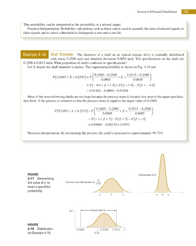
Example 4-16 Shaft Diameter The diameter of a shaft in an optical storage drive is normally distributed
with mean 0.2508 inch and standard deviation 0.0005 inch. The specii cations on the shaft are
±
0.2500 0.0015 inch. What proportion of shafts conforms to specii cations?
Let X denote the shaft diameter in inches. The requested probability is shown in Fig. 4-18 and
.
.
0 2508⎞
0 2508
. (
P 0 2485 < X < 0 2515) = P ⎛ ⎜ ⎝ 0 2485 − . < Z < 0 2515 − . ⎟ ⎠
.
.
0 0 . 0005
0 0005
= ( − 4 6 . < Z < 1 4 . ) = (Z < 1 4 . ) − (Z < − 4 6 . )
P
P
P
=
= 0 91924 −. 0 0000 = 0 91924.
.
Most of the nonconforming shafts are too large because the process mean is located very near to the upper specii ca-
tion limit. If the process is centered so that the process mean is equal to the target value of 0.2500,
.
.
0 2500⎞
. (
0 2500
P 0 2485 < X < 0 2515) = P ⎛ ⎜ ⎝ 0 2485 − . < Z < 0 2515 − . ⎟ ⎠
.
.
0 0005
0 0 . 0005
= ( − 3 < Z < 3) = (Z < 3) − (Z < − 3)
P
P
P
.
= 0 99865. − 0 00135 = 0 9973
.
Practical Interpretation: By recentering the process, the yield is increased to approximately 99.73%.
FIGURE Distribution of N
4-17 Determining N
the value of x to Standardized distribution of 0.45

meet a specified
probability.
– z 0 z – x 0 x

f(x) Specifications

FIGURE
4-18 Distribution 0.2485 0.2508 0.2515 x
for Example 4-16. 0.25