Page 145 - Applied statistics and probability for engineers

Section 4-6/Normal Distribution 123

X – m
Distribution of Z =
s

0 1.5 z
Distribution of X

4 7 9 1011 13 16 x
–3 –1.5 –0.5 0 0.5 1.5 3 z
10 13 x
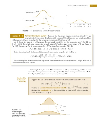
FIGURE 4-15 Standardizing a normal random variable.

Example 4-13 Normally Distributed Current Suppose that the current measurements in a strip of wire are
assumed to follow a normal distribution with a mean of 10 milliamperes and a variance of four
2
(milliamperes) . What is the probability that a measurement exceeds 13 milliamperes?
(
Let X denote the current in milliamperes. The requested probability can be represented as P X > 13). Let
Z = ( X − 10 2. The relationship between the several values of X and the transformed values of Z are shown in
)
Fig. 4-15. We note that X > 13 corresponds to Z > 1 5. Therefore, from Appendix Table III,
.
P X > 13) = ( . 1 P Z ≤ 1 5) = 1 0 93319 = .
P Z > 1 5) = − (
(
0 06681
.
− .
Rather than using Fig. 4-15, the probability can be found from the inequality X > 13. That is,
−
(
P X > 13) = P ⎜ ⎝ ( ⎛ X − 2 10) ( 13 10) ⎞ ⎟ ⎠ = ( 1 5) = .
>
P Z ≤ .
0 06681
2
Practical Interpretation: Probabilities for any normal random variable can be computed with a simple transform to
a standard normal random variable.
In Example 4-13, the value 13 is transformed to 1.5 by standardizing, and 1.5 is often
referred to as the z-value associated with a probability. The following summarizes the calcula-
tion of probabilities derived from normal random variables.
Standardizing
2
to Calculate a Suppose that X is a normal random variable with mean μ and variance σ . Then,
Probability ⎛ X − μ x − μ⎞
(
P Z ≤
P X ≤ x) = P ⎜ ⎝ σ ≤ σ ⎠ ⎟ = ( z) (4-11)
where Z is a standard normal random variable, and z = ( x − μ) is the z-value
σ
obtained by standardizing X. The probability is obtained by using Appendix
Table III with z = ( x − ) μ / s.

x – 10
z = = 2.05
2
FIGURE 4-16 0.98
Determining the
value of x to meet a
specifi ed probability. 10 x