Page 144 - Applied statistics and probability for engineers

122 Chapter 4/Continuous Random Variables and Probability Distributions

(
(
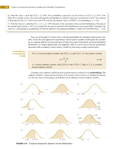
(6) Find the value z such that P Z > z) = .05 . This probability expression can be written as P Z ≤ z) = .95. Now
0
0

Table III is used in reverse. We search through the probabilities to ind the value that corresponds to 0.95. The solution
is illustrated in Fig. 4-14. We do not ind 0.95 exactly; the nearest value is 0.95053, corresponding to z = 1.65.

(7) Find the value of z such that P − ( z < Z < z) = .99. Because of the symmetry of the normal distribution, if the area of
0
the shaded region in Fig. 4-14(7) is to equal 0.99, the area in each tail of the distribution must equal 0.005. Therefore, the
value for z corresponds to a probability of 0.995 in Table III. The nearest probability in Table III is 0.99506 when z = 2.58.
The cases in Example 4-12 show how to calculate probabilities for standard normal random vari-
ables. To use the same approach for an arbitrary normal random variable would require the availabil-
ity of a separate table for every possible pair of values for μ and σ. Fortunately, all normal probability

distributions are related algebraically, and Appendix Table III can be used to ind the probabilities

associated with an arbitrary normal random variable by irst using a simple transformation.
Standardizing a
2
Normal Random If X is a normal random variable with E X ( ) = μ and V X ( ) = σ , the random variable
Variable
X − μ
Z = (4-10)
σ
is a normal random variable with E Z ( ) = 0 and V Z ( ) = 1. That is, Z is a standard
normal random variable.

Creating a new random variable by this transformation is referred to as standardizing. The
random variable Z represents the distance of X from its mean in terms of standard deviations.
It is the key step to calculating a probability for an arbitrary normal random variable.

(1) (5)

= 1 –

0 1.26 0 1.26 –4.6 –3.99 0

(2) (6)
0.05

–0.86 0 0 z > 1.65

(3) (7) 0.99
= 0.005 0.005

–1.37 0 0 1.37 – z 0 z > 2.58

(4)

= –

–1.25 0 0.37 0 0.37 –1.25 0

FIGURE 4-14 Graphical displays for standard normal distributions.