Page 152 - Applied statistics and probability for engineers

130 Chapter 4/Continuous Random Variables and Probability Distributions

0.25 0.4
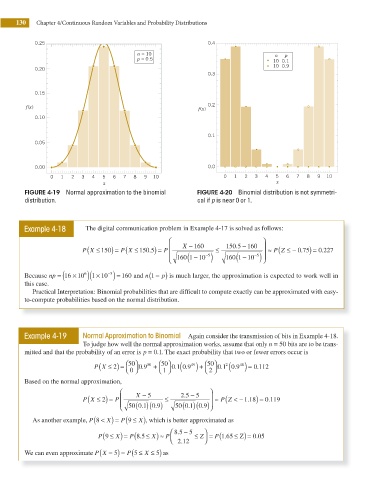
n = 10 n p
p = 0.5 10 0.1
10 0.9
0.20
0.3

0.15
0.2
f(x)
f(x)
0.10

0.1
0.05

0.00 0.0
0 1 2 3 4 5 6 7 8 9 10 0 1 2 3 4 5 6 7 8 9 10
x x
FIGURE 4-19 Normal approximation to the binomial FIGURE 4-20 Binomial distribution is not symmetri-
distribution. cal if p is near 0 or 1.

Example 4-18 The digital communication problem in Example 4-17 is solved as follows:
⎛ ⎛ ⎞
(
P X ≤ 150 5 .
P X ≤ 150 ) = ( ) = P ⎜ X − 160 ≤ 150 5 . − 160 ⎟ ≈ (Z ≤ − 0 75. ) = 0 227.
P
)
⎜ −5 ) −5 ⎟
⎝ 160 − ( 1 10 160 − ( 1 10 ⎠
(
Because np = ( 16 10× 6 )( 1 10× −5 ) = 160 and n 1 − p) is much larger, the approximation is expected to work well in
this case.

Practical Interpretation: Binomial probabilities that are dificult to compute exactly can be approximated with easy-
to-compute probabilities based on the normal distribution.

Example 4-19 Normal Approximation to Binomial Again consider the transmission of bits in Example 4-18.
To judge how well the normal approximation works, assume that only n = 50 bits are to be trans-
.
mitted and that the probability of an error is p = 0 1. The exact probability that two or fewer errors occur is
(
P X ≤ ) = ⎛50 ⎞ 0 9 50 + ⎛50 ⎞ 0. ( 1 0 9. 49 ) + ⎛50 ⎞ 0 1 2 ( 0.9 48 ) = 0..112
.
.
2
⎝ 0 ⎠ ⎝ 1 ⎠ ⎝ 2 ⎠
Based on the normal approximation,
⎛ ⎞
(
.
P X ≤ ) = P ⎜ X − 5 ≤ 2 5 − 5 ⎟ ≈ ( ( − 1 18) = 0 119.
P Z <
2
.
( )( ) ⎠
.
.
( )( ) 9.
⎝
⎜ 50 0 1 0. 50 0 1 0 9 ⎟
(
P 9 ≤
As another example, P 8 < X) = ( X), which is better approximated as
⎞
8 5 −
(
P 9 ≤ X) = ( X) ≈ P ⎛ . 2 12 5 ≤ Z = ( . 0 05
P 1 65 ≤ ) =Z
P 8 5 ≤.
⎜
.
⎟
⎝
⎠
.
(
We can even approximate P X = ) = P(5 ≤ X ≤ ) 5 as
5