Page 157 - Applied statistics and probability for engineers

Section 4-8/Exponential Distribution 135

.
.
. (
.
∫
.
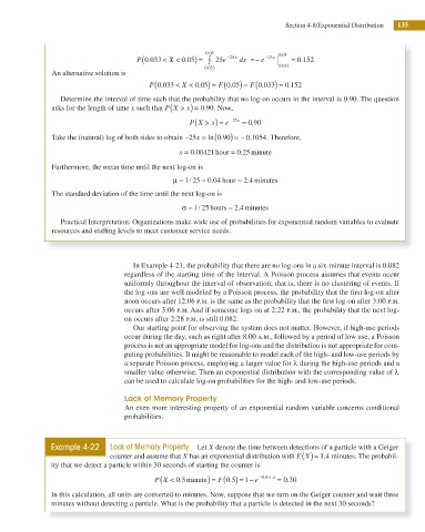
P 0 033 < X < 0 05) = 0 05 25 e − 25 x dx = − e − 25 x 0 05 = 0 1552
.
0 033 0 033
.
An alternative solution is
F 0 05) − (
. (
.
.
.
P 0 033 < X < 0 05) = ( . F 0 033) = 0 152
Determine the interval of time such that the probability that no log-on occurs in the interval is 0.90. The question
(
0
asks for the length of time x such that P X > x) = .90. Now,
(
P X > x) = e −25 x = .90
0
ln
Take the (natural) log of both sides to obtain −25x = (0 . ) = − .1054. Therefore,
90
0
0
0
x = .00421hour = .25 minute
Furthermore, the mean time until the next log-on is
/
μ = 1 25 = .04 hour = .4 minutes
0
2
The standard deviation of the time until the next log-on is
/
σ = 1 25 hours = .4 minutes
2
Practical Interpretation: Organizations make wide use of probabilities for exponential random variables to evaluate

resources and stafing levels to meet customer service needs.
In Example 4-21, the probability that there are no log-ons in a six-minute interval is 0.082
regardless of the starting time of the interval. A Poisson process assumes that events occur
uniformly throughout the interval of observation; that is, there is no clustering of events. If

the log-ons are well modeled by a Poisson process, the probability that the irst log-on after
noon occurs after 12:06 p.m. is the same as the probability that the irst log-on after 3:00 p.m.

occurs after 3:06 p.m. And if someone logs on at 2:22 p.m., the probability that the next log-
on occurs after 2:28 p.m. is still 0.082.
Our starting point for observing the system does not matter. However, if high-use periods
occur during the day, such as right after 8:00 a.m., followed by a period of low use, a Poisson
process is not an appropriate model for log-ons and the distribution is not appropriate for com-
puting probabilities. It might be reasonable to model each of the high- and low-use periods by
a separate Poisson process, employing a larger value for λ during the high-use periods and a
smaller value otherwise. Then an exponential distribution with the corresponding value of λ
can be used to calculate log-on probabilities for the high- and low-use periods.
Lack of Memory Property
An even more interesting property of an exponential random variable concerns conditional
probabilities.

Example 4-22 Lack of Memory Property Let X denote the time between detections of a particle with a Geiger
1
counter and assume that X has an exponential distribution with E X ( ) = .4 minutes. The probabil-
ity that we detect a particle within 30 seconds of starting the counter is
( . ) = ( . − 0 5 1 4 = .
.
/
.
F 0 5) = −
P X < 0 5 minute 1 e 0 30
In this calculation, all units are converted to minutes. Now, suppose that we turn on the Geiger counter and wait three
minutes without detecting a particle. What is the probability that a particle is detected in the next 30 seconds?