Page 153 - Applied statistics and probability for engineers

Section 4-7/Normal Approximation to the Binomial and Poisson Distributions 131

4 5 −
.
(
P 4 5 ≤
P 5 ≤ X ≤ 5) = ( . X ≤ . P ⎛ . 2 12 5 ≤ Z ≤ 5 5 − 5⎞ ⎟
5 5) ≈
⎜
⎝
2 12 ⎠
.
.
= ( 0 24 ≤ Z ≤ 0 24. ) = 0 19.
P − .
Z
= P(4 5. ≤ X ≤ 5 5. )
and this compares well with the exact answer of 0.1849.
Practical Interpretation: Even for a sample as small as 50 bits, the normal approximation is reasonable, when p = 0 1. .
(
The correction factor is used to improve the approximation. However, if np or n 1 − p) is
small, the binomial distribution is quite skewed and the symmetric normal distribution is not
a good approximation. Two cases are illustrated in Fig. 4-20.
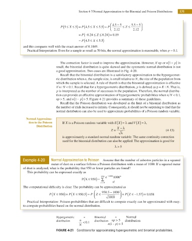
Recall that the binomial distribution is a satisfactory approximation to the hypergeomet-
ric distribution when n, the sample size, is small relative to N, the size of the population from
which the sample is selected. A rule of thumb is that the binomial approximation is effective
if n N/ < 0 1. Recall that for a hypergeometric distribution, p is dei ned as p = K N . That is,
/
.
p is interpreted as the number of successes in the population. Therefore, the normal distribu-
.
tion can provide an effective approximation of hypergeometric probabilities when n N < 0 1,
(
np > 5, and n 1 − p) > 5. Figure 4-21 provides a summary of these guidelines.
Recall that the Poisson distribution was developed as the limit of a binomial distribution as

the number of trials increased to ininity. Consequently, it should not be surprising to ind that the
normal distribution can also be used to approximate probabilities of a Poisson random variable.
Normal Approxima-
tion to the Poisson If X is a Poisson random variable with E X ( ) = λ and V X ( ) = λ ,
Distribution X − λ
Z = (4-13)
λ
is approximately a standard normal random variable. The same continuity correction
used for the binomial distribution can also be applied. The approximation is good for
λ > 5

Example 4-20 Normal Approximation to Poisson Assume that the number of asbestos particles in a squared
meter of dust on a surface follows a Poisson distribution with a mean of 1000. If a squared meter
of dust is analyzed, what is the probability that 950 or fewer particles are found?
This probability can be expressed exactly as
950
(
P X ≤ 950 ) = ∑ e −1000 1000 x
x = 0 ! x

The computational dificulty is clear. The probability can be approximated as
⎛
(
5
P Z ≤ − . ) = .0558
5
P X ≤ 950
P X ≤ 950 ) = ( . ) ≈ P Z ≤ 950 . − 1000 ⎞ ⎟ ⎠ = ( 1 5 7 0
⎜
⎝
1000
Practical Interpretation: Poisson probabilities that are difi cult to compute exactly can be approximated with easy-
to-compute probabilities based on the normal distribution.
Hypergometric ≈ Binomial ≈ Normal
distribution n distribution np > 5 distrribution
< 0 1. _
N n 1( p) > 5
FIGURE 4-21 Conditions for approximating hypergeometric and binomial probabilities.