Page 151 - Applied statistics and probability for engineers

Section 4-7/Normal Approximation to the Binomial and Poisson Distributions 129

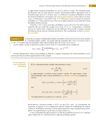
to approximate binomial probabilities for cases in which n is large. The following exam-
ple illustrates that for many physical systems, the binomial model is appropriate with an
extremely large value for n. In these cases, it is difi cult to calculate probabilities by using
the binomial distribution. Fortunately, the normal approximation is most effective in these
cases. An illustration is provided in Fig. 4-19. The area of each bar equals the binomial
probability of x. Notice that the area of bars can be approximated by areas under the normal
probability density function.
(
From Fig. 4-19, it can be seen that a probability such as P 3 ≤ X ≤ 7) is better approxi-
mated by the area under the normal curve from 2.5 to 7.5. Consequently, a modii ed
interval is used to better compensate for the difference between the continuous normal
distribution and the discrete binomial distribution. This modiication is called a continu-

ity correction.

Example 4-17 Assume that in a digital communication channel, the number of bits received in error can be modeled
by a binomial random variable, and assume that the probability that a bit is received in error is
−
×
5
1 10 . If 16 million bits are transmitted, what is the probability that 150 or fewer errors occur?
Let the random variable X denote the number of errors. Then X is a binomial random variable and
150
(
x
,
,
,
−
P X ≤ 150 ) = ∑ ( 16, 000 000 )( 10 −5 ) ( 1 10 −5 ) 16 000 000 − x
x = 0 x
Practical Interpretation: Clearly, this probability is dificult to compute. Fortunately, the normal distribution can be

used to provide an excellent approximation in this example.
Normal Approxima-
tion to the Binomial If X is a binomial random variable with parameters n and p,
Distribution X −
Z = np (4-12)
np(1 − p)
is approximately a standard normal random variable. To approximate a bino-
mial probability with a normal distribution, a continuity correction is applied as
follows:
⎛ − ⎞
(
P X ≤ x) = ( x + 0 5 . ) ≈ P Z ≤ x + 0 5 . np ⎟
P X ≤
⎜
⎜ ⎝ np(1 − p) ⎠ ⎟
and
⎛ − ⎞
(
P x ≤ X) = ( ≤ X) ≈ P ⎜ x − 0 5. np ≤ Z⎟
P x − 0 5.
⎜ ⎝ np(1 − p) ⎟ ⎠
p > 5.
The approximation is good for np > 5and n 1 ( − )

Recall that for a binomial variable X, E X ( ) = np and V X ( ) = np(1 − p). Consequently, the
expression in Equation 4-12 is nothing more than the formula for standardizing the random
variable X. Probabilities involving X can be approximated by using a standard normal distri-
bution. The approximation is good when n is large relative to p.
A way to remember the approximation is to write the probability in terms of ≤ or ≥ and then
add or subtract the 0.5 correction factor to make the probability greater.