Page 132 - Applied statistics and probability for engineers

110 Chapter 4/Continuous Random Variables and Probability Distributions

If X is a continuous random variable, for any x 1 and x 2 ,
(
P x 1 <
P x 1 ≤
P x 1 ≤ X ≤ ) = ( X ≤ ) = ( X < x 2) = ( X < x 2) (4-2)
P x 1 <
x 2
x 2
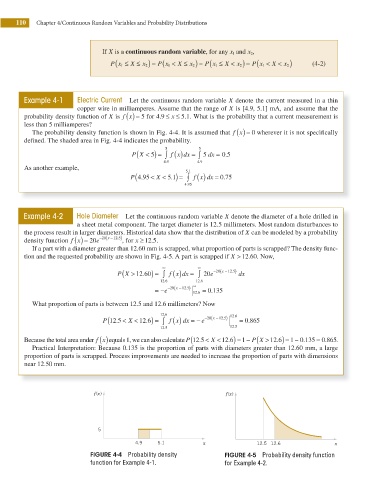
Example 4-1 Electric Current Let the continuous random variable X denote the current measured in a thin
copper wire in milliamperes. Assume that the range of X is [4.9, 5.1] mA, and assume that the
probability density function of X is f x ( ) = 5 for 4 9. ≤ ≤x 5 1. What is the probability that a current measurement is
.
less than 5 milliamperes?
The probability density function is shown in Fig. 4-4. It is assumed that f x ( ) = 0 wherever it is not specii cally
deined. The shaded area in Fig. 4-4 indicates the probability.

(
(
P X < 5) = ∫ 5 f x dx ) = 5 ∫ 5 dx = 0 5
.
4 9 . 4 9
.
As another example, 5 1 .
(
( )
P 4.95 < X < 5.1) = ∫ f x dx = 0 75.
4 95
.
Example 4-2 Hole Diameter Let the continuous random variable X denote the diameter of a hole drilled in
a sheet metal component. The target diameter is 12.5 millimeters. Most random disturbances to
the process result in larger diameters. Historical data show that the distribution of X can be modeled by a probability
. )
− (
density function f x ( ) = 20 e 20 x −12 5 , for x ≥ 12 .5.
If a part with a diameter greater than 12.60 mm is scrapped, what proportion of parts is scrapped? The density func-
tion and the requested probability are shown in Fig. 4-5. A part is scrapped if X > 12.60. Now,
(
(
P X > 12.60) = ∞ ∫ f x dx ) = ∞ ∫ 20 e − ( x − 12 5. ) dx
20
.
.
12 6 12 6
∞
= − e −20( ( x − 12 5. ) 12 6 . = 0 135
.
What proportion of parts is between 12.5 and 12.6 millimeters? Now
.
(
( )
.
P 12.5 < X < 12.6) = 12 6 f x dx = − e − ( x − 12 5. ) 12 6 = .865
20
∫
0
.
.
12 5 12 5
(
P X 12 6) =
−
Because the total area under f x ( ) equals 1, we can also calculate P 12 5. < X <12.6) = − ( > . 1 0 135 = 0 865.
1
.
.
Practical Interpretation: Because 0.135 is the proportion of parts with diameters greater than 12.60 mm, a large
proportion of parts is scrapped. Process improvements are needed to increase the proportion of parts with dimensions
near 12.50 mm.
f(x) f(x)
5
4.9 5.1 x 12.5 12.6 x
FIGURE 4-4 Probability density FIGURE 4-5 Probability density function
function for Example 4-1. for Example 4-2.