Page 191 - Applied statistics and probability for engineers

Section 5-1/Two or More Random Variables 169

With several random variables, we might be interested in the probability distribution of some
…
subset of the collection of variables. The probability distribution of X , X , , X , < p can be
k
k
1
2
…
obtained from the joint probability distribution of X , X , , X p1 2 as follows.
Distribution of a
Subset of Random If the joint probability density function of continuous random variables X , X ,…
2
p)
1
Variables is f X X 2 … ( x , x ,… , x , the probability density function of X , X ,… , X , k < , X p
1 X p 1 2 1 2 k p, is
( … , x k) = … f X X 2 … ( x , x ,… , x p) …
f X X 2 … x , x , ∫ ∫ ∫ 1 2 dx k 1+ dx k 2+ dx p p (5-11)
2
1
1 X k 1 X p
where the integral is over all points R in the range of X , X ,… , X p for which
2
1
X 1 = x , X 2 = x ,… , X k = x k .
2
1
Conditional Probability Distribution
Conditional probability distributions can be developed for multiple random variables by an
extension of the ideas used for two random variables. For example, the joint conditional prob-
ability distribution of X , X , and X given (X = x , X = x ) is
1 2 3 4 4 5 5
( x , x , x 3) = f X X X X X 5 ( x , x , x , x , x 5) X X ( 5) 0.
1
2
3
4
1 2 3 4
1 2 3 |
4 X x , x
4
f X X X x x 5 1 2 4 ( 5) for f 4 5 4 x , x >
f X 4 5
The concept of independence can be extended to multiple random variables.
Independence
Random variables X , X ,… , X p are independent if and only if
2
1
f X X 2 … ( x , x 2 … , x p) = x 1 ( ) x 2 ( )… f X p ( x p)for all x , x , … x (5-12)
1 X p 1 f X 1 f X 2 1 2 , x p
Similar to the result for only two random variables, independence implies that Equation 5-12
holds for all x , x ,… , x p . If we ind one point for which the equality fails, X , X ,… , X p are

2
1
2
1
not independent. It is left as an exercise to show that if X , X ,… , X p are independent,
2
1
(
1) (
P X p ∈
P X 1 ∈ A , X 2 ∈ A ,… , X p ∈ A p) = ( A P X 2 ∈ )… ( A p)
P X 1 ∈
2
1
A 2
… …
p
2
1
for any regions A , A , , A p1 2 in the range of X , X , , X , respectively.
Example 5-17 In Chapter 3, we showed that a negative binomial random variable with parameters p and r can be
represented as a sum of r geometric random variables X , X ,… , X r . Each geometric random vari-
2
1
able represents the additional trials required to obtain the next success. Because the trials in a binomial experiment are
independent, X , X ,… , X r are independent random variables.
1
2
x 3
3 x 2
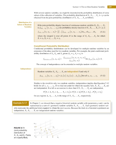
FIGURE 5-11
Joint probability 2 2 3
distribution of 1 1
1 ,
X X 2 , and X 3 . Points 0
are equally likely. 0 1 2 3 x 1