Page 196 - Applied statistics and probability for engineers

174 Chapter 5/Joint Probability Distributions

in short supply in the United States. Although the number of a month without production? Can there be more than one
doses demanded each month is a discrete random variable, the answer? Explain.
large demands can be approximated with a continuous prob- 5-32. The systolic and diastolic blood pressure values (mm
ability distribution. Suppose that the monthly demands for two Hg) are the pressures when the heart muscle contracts and
of those vaccines, namely measles–mumps–rubella (MMR) relaxes (denoted as Y and X, respectively). Over a collection
and varicella (for chickenpox), are independently, normally of individuals, the distribution of diastolic pressure is normal
distributed with means of 1.1 and 0.55 million doses and stand- with mean 73 and standard deviation 8. The systolic pressure is
ard deviations of 0.3 and 0.1 million doses, respectively. Also conditionally normally distributed with mean 1 6. x when X = x
suppose that the inventory levels at the beginning of a given and standard deviation of 10. Determine the following:
month for MMR and varicella vaccines are 1.2 and 0.6 million (a) Conditional probability density function f Y|73 ( y) of Y given
doses, respectively. X = 73
(a) What is the probability that there is no shortage of either (b) P Y <115 | X = 73 )
(
vaccine in a month without any vaccine production? (c) E Y X( | = 73 )
(b) To what should inventory levels be set so that the prob- (d) Recognize the distribution f XY ( x y), and identify the mean
ability is 90% that there is no shortage of either vaccine in and variance of Y and the correlation between X and Y

5-2 Covariance and Correlation

When two or more random variables are dei ned on a probability space, it is useful to describe
how they vary together; that is, it is useful to measure the relationship between the variables. A
common measure of the relationship between two random variables is the covariance. To dei ne
the covariance, we need to describe the expected value of a function of two random variables
, (

h X Y). The deinition simply extends the one for a function of a single random variable.
Expected Value of a
Function of Two ⎧ ∑ ∑ h x, y f XY ( x, y )
(
)
⎪
⎡
Random Variables E h X,Y ( )⎤ = ⎨ X,Y discrete (5-13)
⎦
⎣
)
(
⎩ ⎪ ∫∫ h x, y f XY ( x, ) dx dy X,Y continuous
y
, (
, (
⎡
That is, E h X Y)⎤ can be thought of as the weighted average of h x y) for each point in
⎣
⎦
, (
, (
, (
⎡
the range of X Y). The value of E h X Y)⎤ represents the average value of h X Y) that is
⎦
⎣
expected in a long sequence of repeated trials of the random experiment.
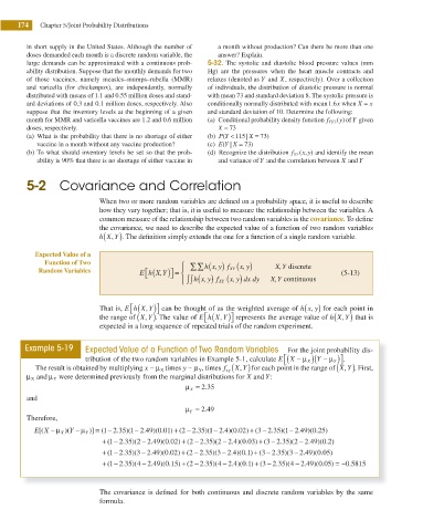
Example 5-19 Expected Value of a Function of Two Random Variables For the joint probability dis-
tribution of the two random variables in Example 5-1, calculate E X − μ )( Y − μ )⎤.
( ⎡
⎣
⎦
X
Y
, (
The result is obtained by multiplying x − μ X times y − μ Y , times f xy( X Y) for each point in the range of X Y). First,
,
μ X and μ Y were determined previously from the marginal distributions for X and Y:
μ = .35
2
X
and
.
μ = 2 49
Y
Therefore,
−
+
.
+
E X − μ X )( Y − μ Y )] = ( − .35 )( − .49 )( .01 ) ( − .35 )( − .4 )( .02) ( 3 2 35 1 2 49 0 25)
.
−
.
1
2
0
2
2
1
1
0
2
)(
2
)(
2
[(
+ ( 1 2 35 2 2 49 0 02) ( 2 2 35)(2 2 4 )(0 03 ) (3 2 35 )(2 2 49 )(0 2 )
−
.
.
.
.
.
−
−
.
−
−
.
.
+
−
.
+
)
(
(
)
(
+ (1 2 35 )(3 2 49 )(0 02) ( − .35 )( − .4 )( .1 ) ( − .35 )( − .49 )( .05 )
+
.
−
.
.
+
−
3
3
2
)
0
0
2
3
2
2
2
.
.
−
+ ( − .35 )( − 2 49 0 15 + ( 2 2 35 4 2 4 0 1 + ( 3 2 35 4 2 49 0 05 = −0 5815
.
.
.
−
.
−
.
.
−
.
0
)(
2
)
)
)(
1
)(
)
)(
4
2
)(
The covariance is dei ned for both continuous and discrete random variables by the same
formula.