Page 200 - Applied statistics and probability for engineers

178 Chapter 5/Joint Probability Distributions

y
4

3
1
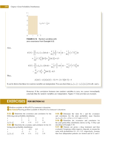
f XY (x,y) = xy
16
2
1

0 1 2 x
FIGURE 5-15 Random variables with
zero covariance from Example 5-22.

Also,
4 2 1 4 2 1 4
)
∫
E X ( ) = ∫ ∫ x f XY ( x, y dx dy = ∫ y x dx dy = ∫ ∫ y x 3 2 dy
3
2
0 0 16 0 0 16 0 0
1
= 1 y 2 2 4 [ ] = [16 2 ] = 4 3
8 3
16 0 6
4 2 4 2 4 2
)
E Y ( ) = ∫ ∫ ∫ y f XY ( x, y dx dy = 1 ∫ y 2 ∫ x dx dy = 1 ∫ y x 2 dy
2
2
0 0 16 0 0 16 0 0
1
= 2 y 3 3 4 = [64 3 ] = 8 3
16 0 8
Thus,
(
E XY) − ( ) ( ) = 32 9/ − (4 3 )(8 3/ ) = 0
/
E X E Y
It can be shown that these two random variables are independent. You can check that f XY ( x, y) = ( ) (
x f y) for all x and y.
Y
f X
However, if the correlation between two random variables is zero, we cannot immediately
conclude that the random variables are independent. Figure 5-12(d) provides an example.
EXERCISES FOR SECTION 5-2

Problem available in WileyPLUS at instructor’s discretion.
Tutoring problem available in WileyPLUS at instructor’s discretion.
5-33. Determine the covariance and correlation for the 5-35. Determine the value for c and the covariance
following joint probability distribution: and correlation for the joint probability mass function
x 1 1 2 4 f XY ( x, y) = ( + , , 3 and y =1 , , 3.
c x y) for x =1
2
2
y 3 4 5 6 5-36. Determine the covariance and correlation for
f XY ( x, y) 1 8 1 4 1 2 1 8 the joint proba.bility distribution shown in Fig. 5-10(a) and
/
/
/
/
5-34. Determine the covariance and correlation for the fol- described in Example 5-10.
lowing joint probability distribution: 5-37. Patients are given a drug treatment and then
x –1 –0.5 0.5 1 evaluated. Symptoms either improve, degrade, or remain the
y –2 –1 1 2 same with probabilities 0.4, 0.1, 0.5, respectively. Assume
f XY ( x, y) 1 8 1 4 1 2 1 8 that four independent patients are treated and let X and Y
/
/
/
/