Page 202 - Applied statistics and probability for engineers

180 Chapter 5/Joint Probability Distributions

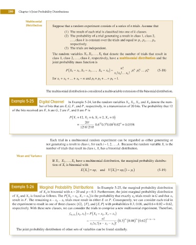
Multinomial
Distribution Suppose that a random experiment consists of a series of n trials. Assume that
(1) The result of each trial is classiied into one of k classes.

(2) The probability of a trial generating a result in class 1, class 2,
… , class k is constant over the trials and equal to p , p ,… , p k ,
1
2
respectively.
(3) The trials are independent.
The random variables X , X ,… , X that denote the number of trials that result in
k
1
2
class 1, class 2, … , class k, respectively, have a multinomial distribution and the
joint probability mass function is
n!
(
P X 1 = x , X 2 = x ,… , X k = x k) = x x 2 !… x k ! p p 2 x 2 … p k x k (5-18)
x 1
2
1
1 !
1
for x 1 + x 2 + …+ x k = n and p 1 + p 2 +…+ p k = 1.
The multinomial distribution is considered a multivariable extension of the binomial distribution.
Example 5-25 Digital Channel In Example 5-24, let the random variables X , X , X 3 , and X 4 denote the num-
1
2
ber of bits that are E, G, F, and P, respectively, in a transmission of 20 bits. The probability that 12
of the bits received are E, 6 are G, 2 are F, and 0 are P is
(
P X 1 = 12 , X 2 = 6 , X 3 = 2 , X 4 = 0)
= 20 ! . 0 6 0 .3 0 .08 0 .02 0 = . 0 0358
6
2
12
12 6 2
! ! ! ! 0
Each trial in a multinomial random experiment can be regarded as either generating or
=
2
not generating a result in class i, for each i , , . . . , k. Because the random variable X i is the
1
number of trials that result in class i, X i has a binomial distribution.
Mean and Variance
If X , X ,… , X k have a multinomial distribution, the marginal probability distribu-
2
1
tion of X i is binomial with
E X i ( ) = np i and V X i ( ) = np i(1 − p i) (5-19)

Example 5-26 Marginal Probability Distributions In Example 5-25, the marginal probability distribution
.
of X 2 is binomial with n = 20 and p = 0 3. Furthermore, the joint marginal probability distribution
(
3 =
2 =
of X 2 and X 3 is found as follows. The P X x , X x 3) is the probability that exactly x 2 trials result in G and that x 3
2
result in F. The remaining n − x − x 3 trials must result in either E or P. Consequently, we can consider each trial in
2
+
G
F
the experiment to result in one of three classes: { }, { }, and {E, P } with probabilities 0.3, 0.08, and 0.6 0.02 = 0.62,
respectively. With these new classes, we can consider the trials to comprise a new multinomial experiment. Therefore,
( x , x 3) = ( = x 3)
P X 2 =
2
2
2
f X X 3 x , X 3
. )
= ! n 0 3 x 2 . ) (0 62 n − x 2 − x 3
x 3
. ( ) (0 08
! !(n
x 3
x x 3 − x 2 − )!
2
The joint probability distribution of other sets of variables can be found similarly.