Page 203 - Applied statistics and probability for engineers

Section 5-3/Common Joint Distributions 181

5-3.2 BIVARIATE NORMAL DISTRIBUTION
An extension of a normal distribution to two random variables is an important bivariate probability
distribution. The joint probability distribution can be dei ned to handle positive, negative, or zero
correlation between the random variables.

Example 5-27 Bivariate Normal Distribution At the start of this chapter, the length of different dimensions of an
injection-molded part were presented as an example of two random variables. If the specii cations for X
and Y are 2.95 to 3.05 and 7.60 to 7.80 millimeters, respectively, we might be interested in the probability that a part satisi es

.
.
0
both speciications; that is, P 2 95 <( . X < 3 5, 7 60 < Y < 7 .80 ). Each length might be modeled by a normal distribution.
However, because the measurements are from the same part, the random variables are typically not independent. Therefore,
a probability distribution for two normal random variables that are not independent is important in many applications.
Bivariate Normal
Probability Density The probability density function of a bivariate normal distribution is
Function
f XY ( x, y; σ X , σ Y , μ X , μ Y , ρ) = 1
2 πσ X σ Y 1 − ρ 2
⎧ ⎡ ( x − μ X) 2 2 ρ( x − μ X y )( − Y μ ) ( y − Y μ ) ⎪
⎤⎫
2
⎪
× exp ⎨ − 1 ⎢ 2 X − + 2 ⎥ ⎬ (5-20)
2
⎪
⎪ ( 2 1 − ρ ) ⎢ ⎣ σ X σ X σ Y Y σ ⎥ ⎦⎭
⎩
for −∞ < x < ∞ and − ∞ < y < ∞, with parameters s . 0, s . 0, − ∞ < μ X < ∞,
Y
X
1
− ∞ < μ Y < ∞, and 2 ,r,1.
,

The result that f XY ( x y;σ X ,σ Y ,μ X ,μ Y , )ρ integrates to 1 is left as an exercise. Also, the
bivariate normal probability density function is positive over the entire plane of real numbers.
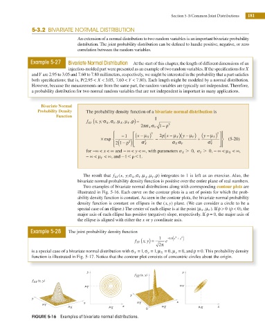
Two examples of bivariate normal distributions along with corresponding contour plots are
illustrated in Fig. 5-16. Each curve on the contour plots is a set of points for which the prob-
ability density function is constant. As seen in the contour plots, the bivariate normal probability
y
density function is constant on ellipses in the ( , ) plane. (We can consider a circle to be a
x
special case of an ellipse.) The center of each ellipse is at the point (μ , μ Y ). If ρ > 0 ( ρ < 0), the
X
major axis of each ellipse has positive (negative) slope, respectively. If ρ = 0, the major axis of
the ellipse is aligned with either the x or y coordinate axis.
Example 5-28 The joint probability density function
2
f XY ( x, y ) = 1 e − . ( 5 x + )
2
0
y
2 π
is a special case of a bivariate normal distribution with σ X = 1, σ y = 1, μ X = 0, μ y = 0, and ρ = 0. This probability density
function is illustrated in Fig. 5-17. Notice that the contour plot consists of concentric circles about the origin.
y y
(x, y)
f XY
(x, y)
f f XY (x, y)
XY
m Y m Y
y
y
x m Y x
m Y
m X m X x 0 m X m X x
FIGURE 5-16 Examples of bivariate normal distributions.