Page 199 - Applied statistics and probability for engineers

Section 5-2/Covariance and Correlation 177

1
0
2
2
E X ( ) = × . + × . + × . + × . = .8
0
0
0
4
1
3
2
0
2
2 2 2 2
.
− . ) × . + (1 1 8
1
− . ) × . + (3
0 2
8
4
V X ( ) = ( 0 0 1 8 0 2 − . ) × . + (2 1 8 0 2 − . ) × . = 1 36
0
1
Because the marginal probability distribution of Y is the same as for X, E Y ( ) = 1 8 and V Y ( ) = 1 36. Consequently,
.
.
Y
E
Y
E
X
1
8
1
8
4
5
1
X
= ( ) − ( ) ( ) = . − . ( ) . ( ) = .26
E
σ XY
Furthermore,
. 1 26
σ XY
= = = .926
0
ρ XY
σ σ Y . 1 36 1 .36
X
Example 5-22 Correlation Suppose that the random variable X has the following distribution: P X ( = ) = 0 2,
1
.
(
P X ( = ) =2 0 6, P X = ) =3 0 2. Let Y = 2 X + 5. That is, P Y = ) = 2, P Y ( = ) = 0 2. Determine
(
.
.
0
7
.
.
11
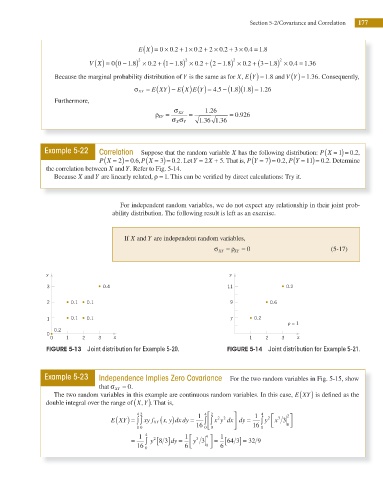
the correlation between X and Y. Refer to Fig. 5-14.
Because X and Y are linearly related, ρ = 1. This can be veriied by direct calculations: Try it.

For independent random variables, we do not expect any relationship in their joint prob-
ability distribution. The following result is left as an exercise.
If X and Y are independent random variables,
σ XY = ρ XY = 0 (5-17)
y y
3 0.4 11 0.2
2 0.1 0.1 9 0.6
1 0.1 0.1 7 0.2
r = 1
0.2
0
0 1 2 3 x 1 2 3 x
FIGURE 5-13 Joint distribution for Example 5-20. FIGURE 5-14 Joint distribution for Example 5-21.
Example 5-23 Independence Implies Zero Covariance For the two random variables in Fig. 5-15, show
= 0.
that σ XY
(

The two random variables in this example are continuous random variables. In this case, E XY) is deined as the
, (
double integral over the range of X Y). That is,
⎤
)
(
⎤
2
E XY) = 4 2 ∫ ∫ xy f XY ( x, y dx dy = 1 ∫ 4 ⎡ ⎢∫ 2 x y dx dy = 1 ∫ 4 y 2 ⎡ ⎣ ⎢ x x 3
3
2 2
⎥
0 ⎦ ⎥
0 0 16 0 ⎣0 ⎦ 16 0
1
[
= 1 ∫ 4 y 8 3] dy = 1 ⎡ y 3 4 ⎤ = [ 64 3] = 32 9
3
2
16 0 6 ⎣ ⎢ 0 ⎦ ⎥ 6