Page 275 - Applied statistics and probability for engineers

Section 7-3/General Concepts of Point Estimation 253

some of the standard probability distributions, such as the exponential and Weibull dis-
tributions. A relatively new computer-intensive technique, the bootstrap, can be used to
solve this problem.
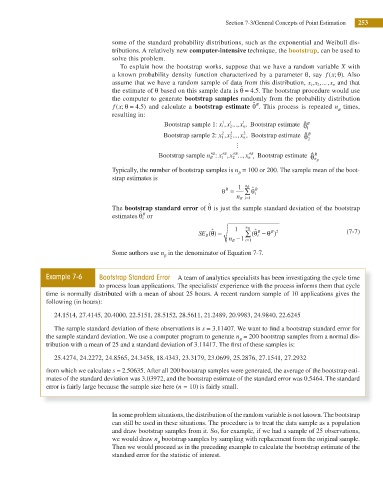
To explain how the bootstrap works, suppose that we have a random variable X with
a known probability density function characterized by a parameter θ, say f x( ; )θ . Also
assume that we have a random sample of data from this distribution, x x 2 , ... , and that
1 ,
x n
ˆ
the estimate of θ based on this sample data is θ = 4 . . The bootstrap procedure would use
5
the computer to generate bootstrap samples randomly from the probability distribution
ˆ B
5
(
f x; θ = 4 . ) and calculate a bootstrap estimate θ . This process is repeated n times,
B
resulting in:
1
1
1 θ
1 ,
Bootstrap sample 1: x x 2 ..., x n 1 , Bootstrap estimate ^ B
2
2
1 ,
Boootstrap sample 2: x x 2 ..., x n 2 , Bootstrap estimate ^ B 2 θ
⋮
nB nB nB nB
B Bootstrap sample n B : x 1 , x 2 ..., x n , Bootstrap estimmate ^ B
θn
B
Typically, the number of bootstrap samples is n = 100 or 200. The sample mean of the boot-
B
strap estimates is
n B
θ = 1 ∑ θ i B ˆ
B
n B i=1
ˆ
The bootstrap standard error of θ is just the sample standard deviation of the bootstrap
ˆ B
estimates θ i or
∑
B ˆ
SE B (θ) = 1 n B (θ i − θ ) (7-7)
ˆ
B 2
n B −1 i=1
Some authors use n in the denominator of Equation 7-7.
B
Example 7-6 Bootstrap Standard Error A team of analytics specialists has been investigating the cycle time
to process loan applications. The specialists' experience with the process informs them that cycle
time is normally distributed with a mean of about 25 hours. A recent random sample of 10 applications gives the
following (in hours):
24.1514, 27.4145, 20.4000, 22.5151, 28.5152, 28.5611, 21.2489, 20.9983, 24.9840, 22.6245
The sample standard deviation of these observations is s = 3.11407. We want to i nd a bootstrap standard error for
the sample standard deviation. We use a computer program to generate n = 200 bootstrap samples from a normal dis-
B

tribution with a mean of 25 and a standard deviation of 3.11417. The irst of these samples is:
25.4274, 24.2272, 24.8565, 24.3458, 18.4343, 23.3179, 23.0699, 25.2876, 27.1541, 27.2932
from which we calculate s = 2.50635. After all 200 bootstrap samples were generated, the average of the bootstrap esti-
mates of the standard deviation was 3.03972, and the bootstrap estimate of the standard error was 0.5464. The standard
error is fairly large because the sample size here (n = 10) is fairly small.

In some problem situations, the distribution of the random variable is not known. The bootstrap
can still be used in these situations. The procedure is to treat the data sample as a population
and draw bootstrap samples from it. So, for example, if we had a sample of 25 observations,
we would draw n bootstrap samples by sampling with replacement from the original sample.
B
Then we would proceed as in the preceding example to calculate the bootstrap estimate of the
standard error for the statistic of interest.