Page 272 - Applied statistics and probability for engineers

250 Chapter 7/Point Estimation of Parameters and Sampling Distributions

ˆ
When an estimator is unbiased, the bias is zero; that is, E( )Θ − θ = .0

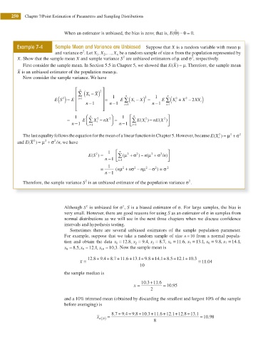
Example 7-4 Sample Mean and Variance are Unbiased Suppose that X is a random variable with mean μ
2 …
and variance σ . Let X , X , , X n1 2 be a random sample of size n from the population represented by
2
2
X. Show that the sample mean X and sample variance S are unbiased estimators of μ and σ , respectively.
First consider the sample mean. In Section 5.5 in Chapter 5, we showed that E X( ) = μ. Therefore, the sample mean
X is an unbiased estimator of the population mean μ.
Now consider the sample variance. We have

⎡ n 2 ⎤
⎢∑ X i ( − X) ⎥ n n
∑
∑
2
=
E S ( ) = E ⎢ i 1 ⎥ = 1 E ( X i − X) = 1 E ( X i 2 + X − 2 XX i)
2
2
−
−
⎢ n 1 ⎥ n 1 i 1 n n −1 i=1
=
⎣ ⎢ ⎦ ⎥
⎛
n
n
= 1 E ∑ X i 2 − nX 2 ⎞ ⎟ = 1 ⎡ ⎢ ∑ E X i ) − nE (X 2 ⎤ ⎥
2 2
⎜
)
(
n −1 i ⎝ =1 ⎠ n −1 ⎣ =i 1 ⎦
2
2
2
The last equality follows the equation for the mean of a linear function in Chapter 5. However, because E X i ) = μ + σ
(
2
and E X( 2 ) = μ + σ 2 /n, we have
n
E S ) = 1 ⎡ ⎢ ∑ (μ + σ − n(μ + σ 2 n / ) ⎤ ⎥
2
2
2
2
)
(
−
n 1 ⎣ = ⎦
i 1
σ
= 1 n ( μ + nσ − nμ − σ ) = σ 2
2
2
2
2
−
n 1
Therefore, the sample variance S is an unbiased estimator of the population variance σ .
2
2
2
Although S is unbiased for σ , S is a biased estimator of σ. For large samples, the bias is
2
very small. However, there are good reasons for using S as an estimator of σ in samples from
normal distributions as we will see in the next three chapters when we discuss coni dence
intervals and hypothesis testing.
Sometimes there are several unbiased estimators of the sample population parameter.
For example, suppose that we take a random sample of size n = 10 from a normal popula-
tion and obtain the data x 1 = 12 8, x 2 = 9 4, x 3 = 8 7, x 4 = 11 6, x 5 = 13 1, x 6 = 9 8, x 7 = 14 1,
.
.
.
.
.
.
.
x 8 = 8 5, x 9 = 12 1, x 10 = 10 3. Now the sample mean is
.
.
.
1
5
1
8
8
7
6
4
12 . + . + . +11 . +13 . + . +14 . + . +12 . +10 .3
8
9
1
8
9
x = = 11 .04
10
the sample median is
3
10 . +11 .6
x = = 10 .95
2
and a 10% trimmed mean (obtained by discarding the smallest and largest 10% of the sample
before averaging) is
8 7 9 4 9 8 10 3 11 6 12 1 12 8 13 1. + . + . + . + . + . + . + .
.
x tr 10 ( ) = = 10 98
8