Page 268 - Applied statistics and probability for engineers

246 Chapter 7/Point Estimation of Parameters and Sampling Distributions

z = 95 −100 = − . 2 5
2
and therefore,
(
P Z < 2 5)
P X < 95) = ( − .
0
= .0062
Practical Conclusion: This example shows that if the distribution of resistance is normal with mean 100 ohms and
standard deviation of 10 ohms, i nding a random sample of resistors with a sample mean less than 95 ohms is a rare
event. If this actually happens, it casts doubt as to whether the true mean is really 100 ohms or if the true standard
deviation is really 10 ohms.

The following example makes use of the central limit theorem.

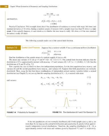
Example 7-2 Central Limit Theorem Suppose that a random variable X has a continuous uniform distribution

⎧1 2/ , 4 ≤ x ≤ 6
f x ( ) = ⎨
⎩ 0, otherwise
Find the distribution of the sample mean of a random sample of size n = 40.
The mean and variance of X are μ = 5 and σ = (6 4 2 12 = 1 3. The central limit theorem indicates that the
2
/
− ) /
2
2
/
distribution of X is approximately normal with mean μ = 5 and variance σ = σ / n = 1 / [ 3 40)] = 1 120. See the
(
X
X
distributions of X and X in Fig. 7-5.

Now consider the case in which we have two independent populations. Let the irst population have mean μ 1 and
2 2
variance σ 1 and the second population have mean μ 2 and variance σ 2 . Suppose that both populations are normally
distributed. Then, using the fact that linear combinations of independent normal random variables follow a normal
distribution (see Chapter 5), we can say that the sampling distribution of X 1 − X 2 is normal with mean
μ = μ − μ (7-2)
1
X 1 −X 2 X 1 X 2 = μ − μ 2
and variance
2 2
σ 2 = σ + σ 2 = σ 1 + σ 2 (7-3)
2
X 1 − X 2 X 1 X 2
n 1 n 2
4 5 6 x
= 1/120
= 2 X
X
95 100 x 4 5 6 x

FIGURE 7-4 Probability for Example 7-1. FIGURE 7-5 The distribution of X and X for Example 7-2.

If the two populations are not normally distributed and if both sample sizes n 1 and n 2 are
more than 30, we may use the central limit theorem and assume that X 2 and X 2 follow approxi-
mately independent normal distributions. Therefore, the sampling distribution of X 1 − X 2 is
approximately normal with mean and variance given by Equations 7-2 and 7-3, respectively.