Page 265 - Applied statistics and probability for engineers

Section 7-2/Sampling Distributions and the Central Limit Theorem 243

2
distributed random variable with mean μ and variance σ . Then because linear functions of
independent, normally distributed random variables are also normally distributed (Chapter 5),
we conclude that the sample mean X + X + … +
X = 1 2 X n
n
has a normal distribution with mean
μ + μ + … + μ
μ = = μ
X
n
and variance
σ + σ + … + σ 2 σ 2
2
2
2 = =
σ X 2
n n
If we are sampling from a population that has an unknown probability distribution, the
sampling distribution of the sample mean will still be approximately normal with mean μ and
2
variance σ / n if the sample size n is large. This is one of the most useful theorems in statistics,
called the central limit theorem. The statement is as follows:
Central Limit
Theorem If X X 2 ,… , X n is a random sample of size n taken from a population (either inite or
1 ,
2
ininite) with mean μ and inite variance σ and if X is the sample mean, the limiting
form of the distribution of
X − μ
Z = (7-1)
σ / n
as n → ∞, is the standard normal distribution.

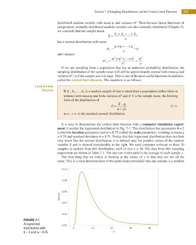
It is easy to demonstrate the central limit theorem with a computer simulation experi-
ment. Consider the lognormal distribution in Fig. 7-1. This distribution has parameters θ = 2
(called the location parameter) and ω = 0.75 (called the scale parameter), resulting in mean μ
= 9.79 and standard deviation σ = 8.51. Notice that this lognormal distribution does not look
very much like the normal distribution; it is deined only for positive values of the random
variable X and is skewed considerably to the right. We used computer software to draw 20
samples at random from this distribution, each of size n = 10. The data from this sampling
experiment are shown in Table 7-1. The last row in this table is the average of each sample x.
The irst thing that we notice in looking at the values of x is that they are not all the
same. This is a clear demonstration of the point made previously that any statistic is a random

0.10

0.08

0.06
Density

0.04

0.02
FIGURE 7-1
A lognormal 0.00
distribution with 0 10 20 30 40
θ = 2 and ω = 0.75. X