Page 267 - Applied statistics and probability for engineers

Section 7-2/Sampling Distributions and the Central Limit Theorem 245

99

95
90
Percent normal probability 70
80
60
50
40
30
20

10
5

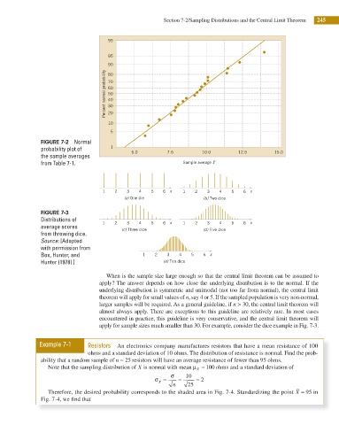
FIGURE 7-2 Normal
probability plot of 1 5.0 7.5 10.0 12.5 15.0
the sample averages
from Table 7-1. Sample average x

1 2 3 4 5 6 x 1 2 3 4 5 6 x
(a) One die (b) Two dice

FIGURE 7-3
Distributions of
1 2 3 4 5 6 x 1 2 3 4 5 6 x
average scores
(c) Three dice (d) Five dice
from throwing dice.
Source: [Adapted
with permission from
Box, Hunter, and 1 2 3 4 5 6 x
Hunter (1978).] (e) Ten dice

When is the sample size large enough so that the central limit theorem can be assumed to
apply? The answer depends on how close the underlying distribution is to the normal. If the
underlying distribution is symmetric and unimodal (not too far from normal), the central limit
theorem will apply for small values of n, say 4 or 5. If the sampled population is very non-normal,
larger samples will be required. As a general guideline, if n > 30, the central limit theorem will
almost always apply. There are exceptions to this guideline are relatively rare. In most cases
encountered in practice, this guideline is very conservative, and the central limit theorem will
apply for sample sizes much smaller than 30. For example, consider the dice example in Fig. 7-3.

Example 7-1 Resistors An electronics company manufactures resistors that have a mean resistance of 100
ohms and a standard deviation of 10 ohms. The distribution of resistance is normal. Find the prob-
ability that a random sample of n = 25 resistors will have an average resistance of fewer than 95 ohms.
Note that the sampling distribution of X is normal with mean μ = 100 ohms and a standard deviation of
X
σ 10
σ = = = 2
X
n 25
Therefore, the desired probability corresponds to the shaded area in Fig. 7-4. Standardizing the point X = 95 in
Fig. 7-4, we i nd that