Page 266 - Applied statistics and probability for engineers

244 Chapter 7/Point Estimation of Parameters and Sampling Distributions

variable. If we had calculated any sample statistic (s, the sample median, the upper or lower
quartile, or a percentile), they would also have varied from sample to sample because they are
random variables. Try it and see for yourself.
According to the central limit theorem, the distribution of the sample average x is normal.
Figure 7-2 is a normal probability plot of the 20 sample averages x from Table 7-1. The
observations scatter generally along a straight line, providing evidence that the distribution of
the sample mean is normal even though the distribution of the population is very non-normal.
This type of sampling experiment can be used to investigate the sampling distribution of any
statistic.
The normal approximation for X depends on the sample size n. Figure 7-3(a) is the distri-
bution obtained for throws of a single, six-sided true die. The probabilities are equal (1 / 6) for
all the values obtained: 1, 2, 3, 4, 5, or 6. Figure 7-3(b) is the distribution of the average score
obtained when tossing two dice, and Fig. 7-3(c), 7-3(d), and 7-3(e) show the distributions of
average scores obtained when tossing 3, 5, and 10 dice, respectively. Notice that, although the
population (one die) is relatively far from normal, the distribution of averages is approximated
reasonably well by the normal distribution for sample sizes as small as ive. (The dice throw
distributions are discrete, but the normal is continuous.)
The central limit theorem is the underlying reason why many of the random variables
encountered in engineering and science are normally distributed. The observed variable of the
results from a series of underlying disturbances that act together to create a central limit effect.

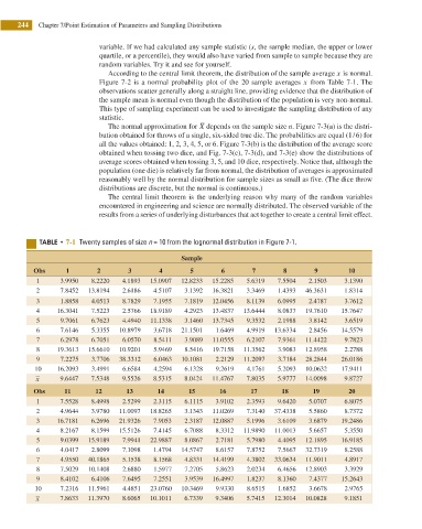
5"#-& t 7-1 Twenty samples of size n = 10 from the lognormal distribution in Figure 7-1.
Sample
Obs 1 2 3 4 5 6 7 8 9 10
1 3.9950 8.2220 4.1893 15.0907 12.8233 15.2285 5.6319 7.5504 2.1503 3.1390
2 7.8452 13.8194 2.6186 4.5107 3.1392 16.3821 3.3469 1.4393 46.3631 1.8314
3 1.8858 4.0513 8.7829 7.1955 7.1819 12.0456 8.1139 6.0995 2.4787 3.7612
4 16.3041 7.5223 2.5766 18.9189 4.2923 13.4837 13.6444 8.0837 19.7610 15.7647
5 9.7061 6.7623 4.4940 11.1338 3.1460 13.7345 9.3532 2.1988 3.8142 3.6519
6 7.6146 5.3355 10.8979 3.6718 21.1501 1.6469 4.9919 13.6334 2.8456 14.5579
7 6.2978 6.7051 6.0570 8.5411 3.9089 11.0555 6.2107 7.9361 11.4422 9.7823
8 19.3613 15.6610 10.9201 5.9469 8.5416 19.7158 11.3562 3.9083 12.8958 2.2788
9 7.2275 3.7706 38.3312 6.0463 10.1081 2.2129 11.2097 3.7184 28.2844 26.0186
10 16.2093 3.4991 6.6584 4.2594 6.1328 9.2619 4.1761 5.2093 10.0632 17.9411
x 9.6447 7.5348 9.5526 8.5315 8.0424 11.4767 7.8035 5.9777 14.0098 9.8727
Obs 11 12 13 14 15 16 17 18 19 20
1 7.5528 8.4998 2.5299 2.3115 6.1115 3.9102 2.3593 9.6420 5.0707 6.8075
2 4.9644 3.9780 11.0097 18.8265 3.1343 11.0269 7.3140 37.4338 5.5860 8.7372
3 16.7181 6.2696 21.9326 7.9053 2.3187 12.0887 5.1996 3.6109 3.6879 19.2486
4 8.2167 8.1599 15.5126 7.4145 6.7088 8.3312 11.9890 11.0013 5.6657 5.3550
5 9.0399 15.9189 7.9941 22.9887 8.0867 2.7181 5.7980 4.4095 12.1895 16.9185
6 4.0417 2.8099 7.1098 1.4794 14.5747 8.6157 7.8752 7.5667 32.7319 8.2588
7 4.9550 40.1865 5.1538 8.1568 4.8331 14.4199 4.3802 33.0634 11.9011 4.8917
8 7.5029 10.1408 2.6880 1.5977 7.2705 5.8623 2.0234 6.4656 12.8903 3.3929
9 8.4102 6.4106 7.6495 7.2551 3.9539 16.4997 1.8237 8.1360 7.4377 15.2643
10 7.2316 11.5961 4.4851 23.0760 10.3469 9.9330 8.6515 1.6852 3.6678 2.9765
x 7.8633 11.3970 8.6065 10.1011 6.7339 9.3406 5.7415 12.3014 10.0828 9.1851