Page 269 - Applied statistics and probability for engineers

Section 7-2/Sampling Distributions and the Central Limit Theorem 247

If either n 1 or n 2 is fewer than 30, the sampling distribution of X 1 − X 2 will still be approxi-
mately normal with mean and variance given by Equations 7-2 and 7-3 provided that the
population from which the small sample is taken is not dramatically different from the normal.
We may summarize this with the following dei nition.

Approximate
Sampling 2
Distribution of a If we have two independent populations with means μ 1 and μ 2 and variances σ 1 and
2
Difference in Sample σ 2 and if X 1 and X 2 are the sample means of two independent random samples of
Means sizes n 1 and n 2 from these populations, then the sampling distribution of
X − X − μ − μ )
2
1
2
( 1
Z = (7-4)
2 2
σ 1 / n + σ 2 / n 2
1
is approximately standard normal if the conditions of the central limit theorem apply.
If the two populations are normal, the sampling distribution of Z is exactly standard
normal.
Example 7-3 Aircraft Engine Life The effective life of a component used in a jet-turbine aircraft engine is a
random variable with mean 5000 hours and standard deviation 40 hours. The distribution of effec-
tive life is fairly close to a normal distribution. The engine manufacturer introduces an improvement into the manufac-
turing process for this component that increases the mean life to 5050 hours and decreases the standard deviation to 30
hours. Suppose that a random sample of n 1 = 16 components is selected from the “old” process and a random sample
of n 2 = 25 components is selected from the “improved” process. What is the probability that the difference in the two
samples means X 2 − X 1 is at least 25 hours? Assume that the old and improved processes can be regarded as independ-
ent populations.
To solve this problem, we irst note that the distribution of X 1 is normal with mean μ = 5000 hours and standard devia-

1
tion σ 1 / 1 n = 40 / 16 = 10 hours, and the distribution of X 2 is normal with mean μ = 5050 hours and standard devi-
2
−
ation σ 2 / 2 n = 30 / 25 = 6 hours. Now the distribution of X 2 − X 1 is normal with mean μ − μ = 5050 5000 = 50
2
1
2
2
2
2
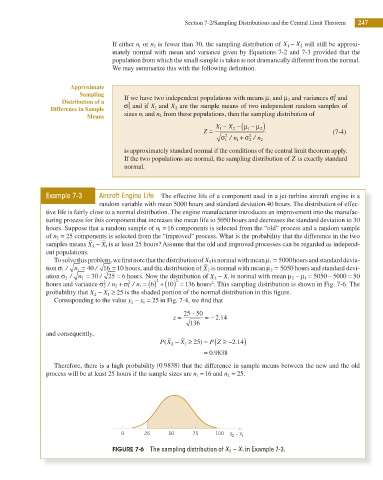
hours and variance σ / n 2 + σ 1 / n = ( 6) +( 10) = 136 hours . This sampling distribution is shown in Fig. 7-6. The
2
2
1
probability that X 2 − X 1 • 25 is the shaded portion of the normal distribution in this i gure.
Corresponding to the value x 2 − x 1 = 25 in Fig. 7-4, we i nd that
z = 25 − 50 = − . 2 14
136
and consequently,
(
P X 2 − X 1 • 25 )= P ≥ − . 2 14)
Z
(
= .
0 9838
Therefore, there is a high probability ( .0 9838 ) that the difference in sample means between the new and the old
process will be at least 25 hours if the sample sizes are n 1 = 16 and n 2 = 25.

0 25 50 75 100 x – x 1
2
FIGURE 7-6 The sampling distribution of X 2 − X 1 in Example 7-3.