Page 283 - Applied statistics and probability for engineers

Section 7-4/Methods of Point Estimation 261

–32.59
0.0
–32.61 –0.1

Log likelihood –32.63 Difference in log likelihood –0.2

–32.65

n = 20
–32.67 –0.3 n = 8
–0.4 n = 40
–32.69
.040 .042 .044 .046 .048 .050 .052 0.038 0.040 0.042 0.044 0.046 0.048 0.050 0.052 0.054
l l
(a) (b)
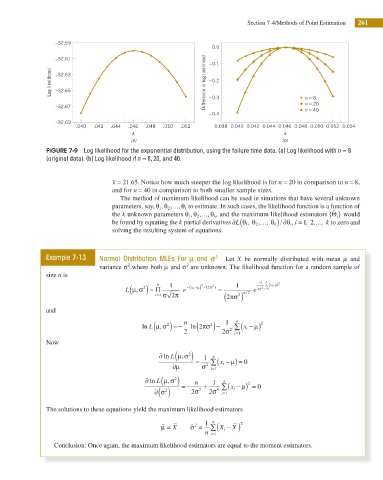
FIGURE 7-9 Log likelihood for the exponential distribution, using the failure time data. (a) Log likelihood with n = 8
(original data). (b) Log likelihood if n = 8, 20, and 40.

x = 21 .65. Notice how much steeper the log likelihood is for n = 20 in comparison to n = 8,
and for n = 40 in comparison to both smaller sample sizes.
The method of maximum likelihood can be used in situations that have several unknown
,
,
,
parameters, say, θ θ … θ k to estimate. In such cases, the likelihood function is a function of
2
1
∧
,
,
,
the k unknown parameters θ θ … θ k , and the maximum likelihood estimators { } would
Q
2
i
1
be found by equating the k partial derivatives ∂ ( θ θ … θ ) ∂θ , i1 , 2 , , k / i = 1 , , , k to zero and
…

L
2
solving the resulting system of equations.
2
Example 7-13 Normal Distribution MLEs For l and r Let X be normally distributed with mean μ and
2
2
variance σ where both μ and σ are unknown. The likelihood function for a random sample of
size n is
L μ ( , ) = Π 1 e −( x i −μ) 2 / 2( σ 2 ) = 1 e 2 −1 n ∑ 1 ( x i −μ) 2 2
n
È
2
2
σ i=
i=1 σ 2 π ( 2 πσ ) n/ 2
2
and
ln ( μ ) = − n ln( 2 πσ ) − 1 ∑ − μ) 2
n
σ
2
2
,
L
2 2 σ 2 = i 1 (x i
Now
2
∂ ln L μ ( , σ ) 1 n
∂μ = σ 2 ∑ (x i − μ) = 0
= i 1
2
∂ ln L μ ( , σ ) n 1 n 2
∂ σ ( ) = − 2 σ 2 + 2 σ 4 ∑ (x i − μ) = 0
2
= i 1
The solutions to these equations yield the maximum likelihood estimators
(
1 n 2
2
X
ˆ μ = X ˆ σ = ∑ X i − )
n = i 1
Conclusion: Once again, the maximum likelihood estimators are equal to the moment estimators.